Key Steps in the Workflow to Analyze Raman Spectra

Raman spectroscopy is based on Raman scattering, an inelastic scattering process that is only observed in a tiny proportion (~1 in 10⁶) of the photons scattered by a molecule. As Raman spectroscopy typically measures the vibrational states, it can be used to characterize the molecular components of the sample, and hence, it provides a unique fingerprint of the sample. The technology is being applied in many scenarios in biology, forensics, diagnostics, pharmaceutics, and food science. Its power is further enhanced by spectral analysis methods, which can extract subtle changes from Raman spectra and translate the fingerprint information to high-level knowledge efficiently. The Raman spectral analysis is composed of three main parts: the experimental design; the preprocessing; and the data modeling (1). In this article, we would like to highlight the 11 key steps to analyze Raman data, which is depicted in Figure 1.

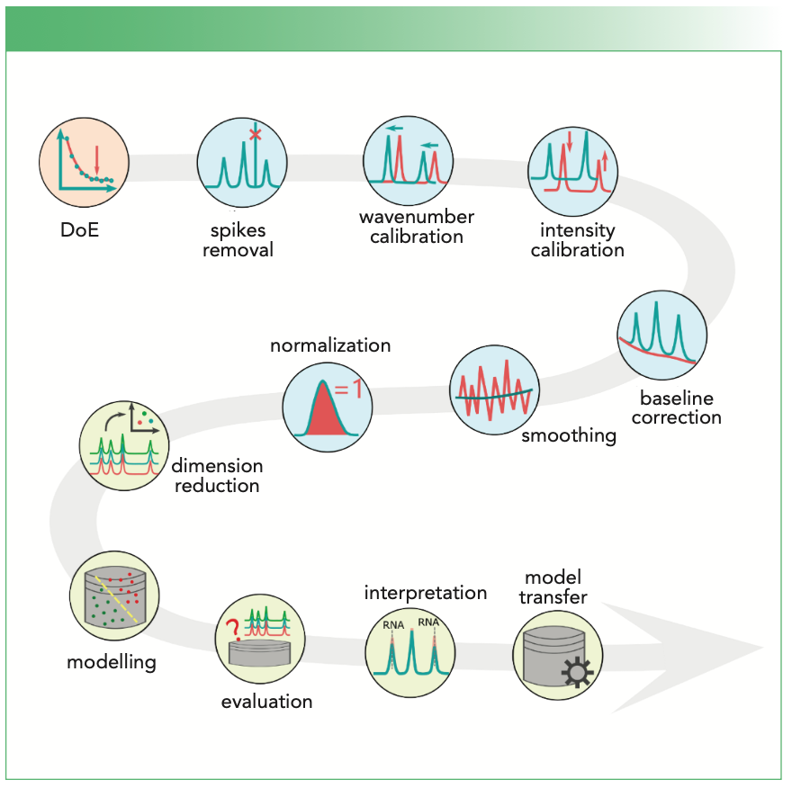
FIGURE 1: The 11 key steps of Raman spectral analysis, which are linked to the main steps: DoE, pre-processing, and modelling.

Experimental Design

Sample Size Planning

Sample size planning (SSP) is the most important step of experimental design (DoE) in the field of Raman spectral analysis. It aims to estimate the minimal number of samples to reach a statistically meaningful conclusion or to build a model with acceptable performance. The term sample refers to the highest level of the sampling hierarchy; for example, it could be a patient, a (biological) batch, or a (biological/technical) replicate. SSP can be achieved based on the learning curve that characterizes a predefined metric over the increasing sample size; look for the minimal sample size where the metric does not improve further (2).

Preprocessing

Measured Raman spectra are not perfect, but are corrupted by different (side) effects originating from the instrument, the environment, and the sample itself. These corrupting effects are removed via a series of preprocessing steps, including quality control, spikes removal, (spectrometer) calibration, baseline correction, smoothing, and normalization. These steps are not independent, but they do impact each other. We recommend putting them into a closed loop and adjusting one step according to the feedback of the other steps.

Spikes Removal

Cosmic spikes occur when high-energy cosmic particles hit the charge coupled device (CCD) or complementary metal oxide semiconductor (CMOS) detector. They manifest themselves as narrow but extremely intense bands, and they can appear randomly at any wavenumber positions. In practice, spikes are normally detected as abnormal intensity changes when comparing two successively measured spectra or screening along the wavenumber axis within one spectrum. Methods are also reported to jointly inspect such intensity changes along the wavenumber axis and between the successive measurements simultaneously (3). The detected spikes are replaced with either an interpolation-based value using the boundary points of the spike position or the intensities of its successive measurement at the same wavenumber positions. In the latter way, the fluorescence and the intensity variations between the two measurements have to be handled well.

The Spectrometer Calibration

The spectrometer calibration is to remove spectral variations caused by the changes in devices and environment so that the spectra become comparable among different measurements. Typically, it involves a wavenumber and intensity calibration (4). Spectra of standard materials are measured in both cases. For wavenumber calibration, the calibration function is estimated by aligning the measured band positions of the wavenumber standard to their theoretical values—for instance, through a polynomial fitting. For the intensity calibration, the intensity response function can be calculated as the ratio between the measured and theoretical emission of an intensity standard. This response function is then used to divide the measured Raman intensities for the calibration.

Baseline Correction

Baseline correction normally refers to the correction of fluorescence of the sample. Fluorescence shows as a slowly changing baseline under Raman bands; this property can be used to correct it. Many mathematical approaches exist for this correction, including derivative spectra, the sensitive nonlinear iterative peak (SNIP) clipping, asymmetric least squares smoothing, polynomial fitting, standard normal variate (SNV), multiplicative scattering correction (MSC), and extended multiplicative signal correction (EMSC).

Smoothing

Smoothing is usually achieved via a moving-window low-pass filtering (for example, mean, median, or Gaussian) in the spectral or spatial domain. The spectral filtering works along the wavenumber axis; hence, it can be applied for a single spectrum. The spatial filtering, in contrast, is calculated over multiple spectra collected from a spatial neighborhood, and thus, it is only applicable in hyperspectral data cubes. In either manner, smoothing may degrade the subsequent analysis and is recommended only for highly noisy data.

Normalization

Normalization is performed to suppress the fluctuation of the excitation intensity or changes in the focusing conditions of the setup. Here, the spectral intensities are divided by the area, maximum, or l₂ norm of a selected spectral region (R), respectively; R, dependent on the task, can be the whole spectrum, a single wavenumber position, or a Raman band with supposedly constant intensities.

Data Modeling

After the data is preprocessed, the spectral signals are translated into high-level information (such as response variables), for instance, the disease status or the concentration of a component. This requires a certain number of samples with known response variables. A statistical or machine learning model is constructed with part of the data set (training data) and evaluated with the rest (testing data). The model with optimal performance is afterward used for unknown samples to obtain their response variables directly. The major steps of statistical or data modeling are explained in the next section.

Dimension Reduction

Dimension reduction helps to extract useful features from the data and reduce redundant information. Depending on whether the response information is needed or not, existent approaches can be categorized as supervised or unsupervised procedures. Typical examples are principal component analysis (PCA) and the partial least squares (PLS), respectively. Dimension reduction can also be grouped into feature selection or feature extraction. Methods for feature selection pick the variables that are the most significant according to a predefined benchmark, whereas feature extraction transforms the spectral data into a new space of lower dimension and represent the original spectra with new coordinates. Typical approaches in such case are PCA, vertex component analysis (VCA), N-Finder, independent component analysis (ICA), and multivariate curve resolution alternative least squares (MCR-ALS) (1).

Model Construction

The output of the dimension reduction is supplied to a machine learning model to translate the spectral signal into high-level information. Existent models can be categorized as unmixing, clustering, classification, or regression. The unmixing and clustering are applicable for image generation and rough data inspection—for example, to see the spatial pattern of a hyperspectral data cube. The classification relates the spectral signals to a categorical variable such as disease status. Regression models derive a quantitative value, such as the concentration of given substances, from the spectral signal. No clear separation exists between classification and regression models; as a matter of fact, classification is often achieved via a regression model.

Model Evaluation

After being constructed, the prediction performance of the model is evaluated with testing data. All supervised procedures contributing to the model prediction should be involved in such an evaluation, be it dimension reduction or the machine learning model itself. The prediction performance is characterized via the deviation of the prediction from the known true values. Examples of performance markers of the models are the root-mean squared-error of prediction (RMSEP) for regression models and accuracy, sensitivity, specificity, selectivity, and Cohen’s kappa for classification models (1). To make better use of the known samples, it is recommended to perform model evaluation in the framework of cross-validation, where the known data is split into training and testing data for multiple times. The predictions over all data splits are averaged to evaluate the performance of the model. In all splits, the testing data must be independent to the training data to avoid model overestimation. That means, the two data sets must be from different patients or batches (5).

Model Interpretation

Model interpretation is another important step in data modeling, which could be performed based on the variable significance indicated by the established model. Variables of the spectroscopic data that are shown to be important to the model should link to chemical or biological explanations. This can help further feature selection to build a more parsimonious model. In the long run, such a model interpretation can help to discover the biomarkers that play a role in the given investigation.

Model Transfer

As sensitive as Raman spectroscopy, it is common to see significant shifts of Raman bands or changes in Raman intensities between spectra measured from different replicates or on different devices. Hence, an established model can perform badly when predicting new data—for instance, Raman spectra measured from a patient to be diagnosed. Model transfer is utilized in this case, which helps to improve the prediction of an existent model on new data. This can be achieved either by either removing the spectral variations between the different measurements or adjusting the model parameters by taking the features of the new data into account (6).

Conclusion

To summarize, we walked through the key steps of the Raman spectral analysis workflow and briefly discussed their aims and available approaches. Possible errors upon misconducting of the steps are summarized in (7). With such a condensed article, we hope to unveil the mystery of Raman spectral analysis so that the results of the analysis are more easily understood and interpreted. For more detailed and comprehensive conceptions of each step, the readers are kindly referred elsewhere (1,8).

Acknowledgment

This work is supported by the BMBF, funding program Photonics Research Germany (FKZ:13N15466 (BT1), FKZ:13N15706 (BT2) FKZ:13N15715 (BT4)) and is integrated into the Leibniz Center for Photonics in Infection Research (LPI). The LPI initiated by Leibniz-IPHT, Leibniz-HKI, UKJ and FSU Jena is part of the BMBF national road map for research infrastructures.

References

(1) Guo, S.; Popp, J.; Bocklitz, T. Chemometric Analysis in Raman Spectroscopy from Experimental Design to Machine Learning–based Modeling. Nat. Protoc. 2021, 16, 5426–5459. DOI: 10.1038/s41596-021-00620-3

(2) Ali, N.; Girnus, S.; Roesch, P.; Popp, J.; Bocklitz, T. W. Sample-Size Planning for Multivariate Data: A Raman-Spectroscopy-Based Example. Anal. Chem. 2018, 90, 12485–12492. DOI: 10.1021/acs.analchem.8b02167

(3) Ryabchykov, O.; Bocklitz, T.; Ramoji, A.; Neugebauer, U.; Foerster, M.; Kroegel, C.; Bauer, M.; Kiehntopf, M.; Popp, Automatization of Spike Correction in Raman Spectra of Biological Samples. J. Chemom. Intell. Lab. Syst. 2016, 155, 1–6. DOI: 10.1016/j.chemolab.2016.03.024

(4) Bocklitz, T. W.; Dörfer, T.; Heinke, R.; Schmitt, M.; Popp, J. Spectrometer Calibration Protocol for Raman Spectra Recorded with Different Excitation Wavelengths. Spectrochim. Acta. A. Mol. Biomol. Spectrosc. 2015, 149, 544–549. DOI: 10.1016/j.saa.2015.04.079

(5) Guo, S.; Bocklitz, T.; Neugebauer, U.; Popp, J. Common Mistakes in Cross-validating Classification Models. Anal. Meth. 2017, 9 (30), 4410–4417. DOI: 10.1039/C7AY01363A

(6) Guo, S.; Kohler, A.; Zimmermann, B.; Heinke, R.; Stöckel, S.; Rösch, P.; Popp, J.: Bocklitz, T. Extended Multiplicative Signal Correction Based Model Transfer for Raman Spectroscopy in Biological Applications. Anal. Chem. 2018, 90 (16), 9787–9795. DOI: 10.1021/acs.analchem.8b01536

(7) Ryabchykov, O.; Schie, I.; Popp, J.; Bocklitz, T. Errors and Mistakes to Avoid when Analyzing Raman Spectra. Spectroscopy 2022, 37 (4), 48–50. DOI: 10.56530/spectroscopy.zz8373x6

(8) Guo, S.; Ryabchykov, O.; Ali, N.; Houhou, R.; T. Bocklitz, T, in Reference Module in Chemistry, Molecular Sciences, and Chemical Engineering; Elsevier, 2020.

Shuxia Guo, Jürgen Popp, and Thomas Bocklitz are with the Leibniz Institute of Photonic Technology in Jena, Germany. Popp and Bocklitz are also with the Friedrich Schiller University in Jena, Germany. Bocklitz is also with the Institute of Computer Science, Faculty of Mathematics, Physics & Computer Science, at the University Bayreuth (UBT), in Bayreuth, Germany. Direct correspondence to: thomas.bocklitz@uni-jena.de ●