Discrimination of Geographical Origin for Purple Sweet Potato Using Hyperspectral Imaging Combined with Multivariate Analysis

The origin and quality of purple sweet potatoes affect several purple sweet potato products, such as purple sweet potato juice and purple sweet potato flour. Because of this, discriminating the geographical origin of purple sweet potatoes is important. In this study, the feasibility of the rapid discrimination of three different geographical origins of purple sweet potato with a hyperspectral imaging (HSI) system was examined. Different chemometrics, including partial least squares–discriminant analysis (PLS-DA), extreme learning machine (ELM), and least squares support vector machines (LS-SVM), combined with principal component analysis (PCA), successive projections algorithm (SPA), and uninformative variable elimination (UVE), were compared to obtain the best discrimination model. The results demonstrated the apparent differences among the three different geographical origins of purple sweet potatoes in fatty acid compositions and the absorbance spectra, and an excellent classification (prediction set false positive rate is 4.598% in prediction set) could be achieved using the LS-SVM method combine with PCA. It can be concluded that hyperspectral imaging with chemometrics can be an effective technique to rapidly discriminate the geographical origin of purple sweet potatoes efficiently.

Purple potato, also known as black potato, is purple or dark purple, rich in vitamins, minerals, carbohydrates, and other nutrients. It is known to have positive health effects, such as anti-inflammatory benefits and liver protection. Purple potato is a variety introduced from abroad. It has been planted on a large scale in China, and various types have been cultivated, all of which have either high nutritional value, significant economic effects, or both. Purple potato is a green health food that can satisfy people’s daily intake of cereals. Affected by weather, altitude, and other factors, purple potato in different producing areas has significant differences in its internal nutrients and nutritional content. In recent years, domestic and foreign research on purple sweet potatoes has mainly focused on its structural identification, extraction, purification, stability, and functional biological activity (1–3). However, geographical origin detection is commonly carried out subjectively by manual inspection, which is costly. Some varieties have no noticeable color change or juice outflow when observed only by the naked eye (4).

Moreover, efficiency and accuracy are significantly reduced after continuous manual inspection. Hence, it is essential to develop a rapid, non-contact detection technique to identify the geographical origin of purple sweet potato. By sorting purple sweet potato using its geographical origin, better quality is realized, yielding a better price with less food waste.

Recently, contactless methods (for example, near-infrared (NIR) spectroscopy and multispectral/hyperspectral imaging (HSI)) that are sensitive to the intramolecular vibrations, involving C-H, O-H, N-H, and possibly S-H and C=O, have been increasingly applied as a powerful analytical tool for rapid determination of food quality. Many of the spectroscopic techniques mentioned above have been widely used in food detection (5–8). Liu Chunquan and others have studied that the internal water content of purple sweet potatoes is 74.57%, and it contains 12.2% starch and 1.2% protein (9). Steed and others (10) reported that the anthocyanin content in American purple sweet potatoes was between 51.5–174.7 mg/100 mg. NIR exhibits obvious disadvantages and although it can accurately determine the internal nutritional content of purple potatoes, it cannot quickly and non-destructively determine the quality of purple potatoes. He Yong and others (11) used mid-infrared (MIR) spectroscopy and chemometric algorithms to identify the origin and varieties of walnuts and achieved good results. However, MIR spectroscopy technology selects spectral information randomly, making it difficult to select the most differentiated spectrum. Hyperspectral technology can select a sensitive area after image processing, and a spectrum measured at the sensitive area can best determine the differences between samples.

Hyperspectral imaging (HSI) is an advanced technology that combines detector systems, precision optics, signal processing, computer science, and information extraction. It is a multi-dimensional information acquisition technology that combines imaging capabilities and spectral measurements. It simultaneously detects the two-dimensional (2D) geometric space of the target and one-dimensional (1D) spectral information to obtain continuous, narrow-band image data with high spectral resolution. The image information can measure external quality characteristics such as the sample size, shape, and observable defects. The spectral information can fully reflect the differences in physical structure and chemical composition inside the sample. Therefore, the spectral image can indicate the overall quality of the sample. The wide variety of spectral characteristics and morphologies of different materials can be determined in fine detail using HSI technology. However, until now, there is no research reported about the application of the hyperspectral technique combined with the chemometric methods for rapid discrimination of the geographical origin of purple sweet potato (12–15).

Spectroscopic techniques, including HSI, have increased in importance for fruit geographical origin detection coupled with multivariate analysis methods. The least squares support vector machines (LS-SVM) model was set up for identifying the subtle varieties of purple sweet potato with the effective wavelengths picked up by principal component analysis (PCA) and successive projections algorithm (SPA) combination methods (16–18). PCA and radial basis function-support vector machine (RBF-SVM) classification was used in vis-NIR HSI for detecting the hidden geographical origin image on purple sweet potato (19). Partial least squares (PLS) method and stepwise discrimination analysis were used for data dimensionality reduction and selecting the effective wavelengths in early detection of geographical origin detection on different background colors using HSI (20–21).

Recently, some studies focused on quality control for fruits, but the selection of geographical origin is the source of high quality fruits (22). To study the geographic origin of purple sweet potato after HSI processing, the most different perceptual area spectrum was selected to maximize the difference, to determine if HSI technology is suitable for the non-destructive detection of the geographic origin of purple sweet potatoes. Collectively, the objectives of this study were to develop a method to discriminate purple sweet potatoes from different geographical origins using hyperspectral spectroscopy combined with different chemometric methods, including partial least squares–discriminant analysis (PLS-DA), extreme learning machine (ELM) and least squares support vector machines (LS-SVM). Meanwhile, the feature selection methods, including PCA, SPA, and uninformative variable elimination (UVE), were also discussed to find the best method to reduce the high dimension of hyperspectral data.

Materials and Methods

Sample Preparation

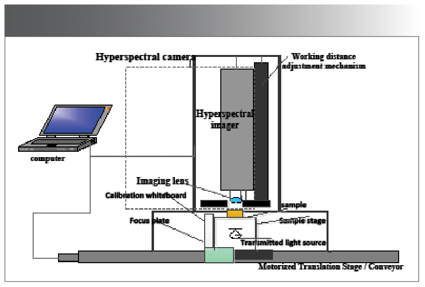
The purple potato samples from this experiment came from three production areas in Guangxi, Fujian, and Shandong. When choosing samples, purple sweet potatoes with similar shapes and sizes, smooth surfaces, and normal type were chosen as the experimental samples. Before the experiment, the samples were simply washed to remove the dirt and impurities on the surface of the purple sweet potatoes. The samples were stored at room temperature for more than 24 h. There are 120 samples in total, including 40 Guangxi purple potatoes, 40 purple potatoes from Fujian, and 40 purple potatoes from Shandong were selected. A total of 120 samples were used for image acquisition by the HSI system (Figure 1).

Figure 1: Schematic of HSI system.

Experimental Instruments

A HSI system was purchased from Sichuan Dualix Spectral Image Technology. The transmission HSI system includes a transmission light source, an imaging spectrometer, a charge-coupled device (CCD) camera, a lens, a displacement platform, a controller, a dark box, and a computer.

Spectra Data Acquisition

Before collecting purple sweet potato images, the HSI system needed to be opened for a warm-up time of approximately 30 min to make it reach a stable working state. After preheating, the computer’s Spectra View software was opened to ensure that the best purple potato image is collected. The relevant parameters of the image acquisition system were then set. Among them, the moving speed of the mobile platform was adjusted to minimize deformation (distortion) of the acquired images. After several experiments and adjustments, the acquisition parameters of the experimental image system were finally determined: the forward speed of the mobile platform was 1 cm/s, the backward speed of the mobile platform was 2.5 cm/s, the exposure time of the camera was 6 ms, and the spectral resolution was 2.8 nm, 26 cm from the mobile platform. Adjusting the camera’s focus was also key to capturing a clear image. The focus window of this image acquisition software displayed three spectral lines composed of red, green, blue (RGB) three colors. The RGB three-color lines have the best sharpness and the most appropriate focal length. Therefore, one can determine whether the system focuses by rotating the camera lens to observe whether the reflection peak at a certain wavelength of the image reaches the best sharpness. By placing the sample on the mobile platform, clicking the acquisition button, and performing the lateral movement, the hyperspectral camera completes the image scanning. This method was used to complete image acquisition for all samples.

The image information was easily affected by the CCD camera’s dark current and uneven illumination during acquisition. To obtain high-quality image information, black and white correction was also required. First, an image of a standard whiteboard (I_W) was captured, and then a cover over the camera lens was to capture a completely dark (black) image (I_B). I_W and I_B were used to correct the original image of the purple sweet potato. The correction formula is as follows (equation 1):

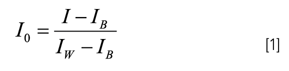
In the formula, I₀ is the corrected purple potato image data, and I is the original purple potato image data.

Data Processing Method

Partial Least Squares (PLS-DA)

PLS is a commonly used method of multivariate data analysis. It finds the best matching function for a set of data by minimizing the square of the error. It is often used to perform regression analysis on the relationship between chemical components and spectral data. In this experiment, this method is used to establish a PLS, qualitative analysis model. The correlation coefficient and root mean square error were used as the main indicators to measure the quality of a model. The greater correlation coefficient and smaller root mean square error (RMSE) are indispensable diagnostics for a good model. The calculation steps of each spectrum X and bruising time Y between T and U are shown in equations 2 and 3:

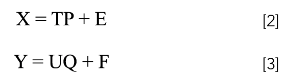
T and U are the score matrices of X and Y, respectively, P and Q are the load matrices of X and Y, respectively, and E and F are the PLS fitting residual matrix of X and Y, respectively. The linear regression equations of T and U are equations 4 and 5.

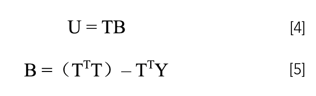
B is the correlation coefficient matrix. In the prediction, the score array T of the unknown sample is obtained from the spectral array X unknown of the unknown sample and the load array P unknown. Then, the collision time of unknown samples can be calculated according to the formula, and the calculation formula is shown in equation 6.

The flow chart of calculation during modeling is shown in Figure 5, and the corresponding matrix factors w, t, p, u, q, and b can be obtained.

During the prediction period, the predicted value of unknown samples can be calculated according to equation 7.

b_K = w_T(pw_T) − 1q is regression coefficient (23,24).

Least Square Support Vector Machine (LS-SVM)

Least squares support vector machine (LS-SVM) is a type of SVM. It is the most suitable for a small sample learning environment For small sample sizes, LS-SVM demonstrates several unique advantages over deep learning algorithms, especially in linear, nonlinear, and high-dimensional pattern recognition tasks. By using the least-squares method, LS-SVM reduces computational requirements. Although deep learning is well-suited for complex pattern recognition problems, it is also a computationally intensive machine learning approach. In this study, which focuses on the supervised classification of yellow peach bruising in real-time, the problem aligns with linear equations, and the data set is small. Under these conditions, LS-SVM processes data significantly faster than deep learning algorithms within a certain data range.

For example, suppose there are N training samples {(X_i, y_i),...,(x_N, y_N)}. Among them, X_i is the input of the n dimensional training sample, y_i is the output of the training sample, and the objective optimization function of the LS-SVM is:

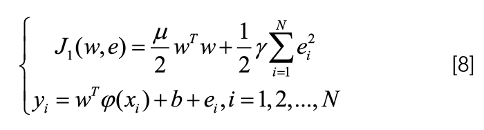
Among them, the mapping function of the kernel space, w is the weight vector; e is the error variable; b is the offset; and µ and y are adjustable parameters.

In order to find the minimum value of the optimization function, construct the Lagrangian function (equation 9):

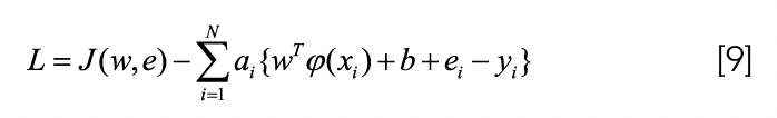
In the formula, a_i is the Lagrange multiplier.

The partial derivative of equation 10 can be obtained:

By eliminating w and e in the formula, the optimization problem can be transformed into solving a linear equation:

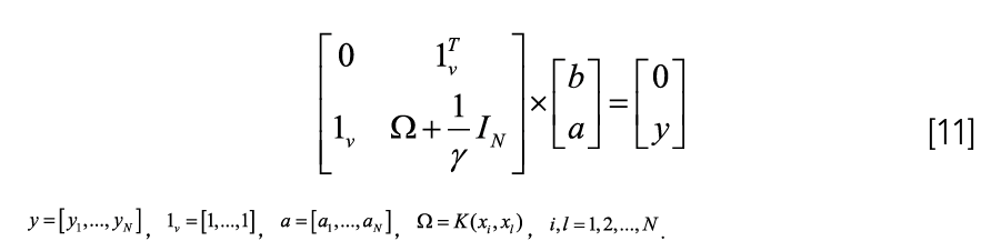
By solving equation (12), a and b can be obtained, and then the LS-SVM used for function estimation is:

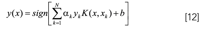
Two standard functions include linear (Lin) and radial basis function (RBF), which are expressed as (13) and (14).

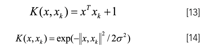
Where σ² is the square of the band width, it is optimized by external optimization techniques during training (25).

Extreme Learning Machine

Extreme learning machine (ELM) is a single hidden layer feedforward neural network algorithm. Its characteristic is that the input weights and the threshold values of hidden layer neurons are randomly selected. In the training process, we only need to adjust the number of neurons in the hidden layer. Figure 2 is the flow chart of the ELM. The input variable is x, the selected excitation function is G(x), the implied weight variable connected to the input node is w, the implied node is L, the bias of the implied node is b, the implied weight connected to the output node is β, and the output variable is f(x) (26). The formula is as follows:

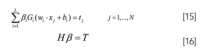
Figure 2: The flow diagram of ELM.

Results and Analysis

Spectra Analysis

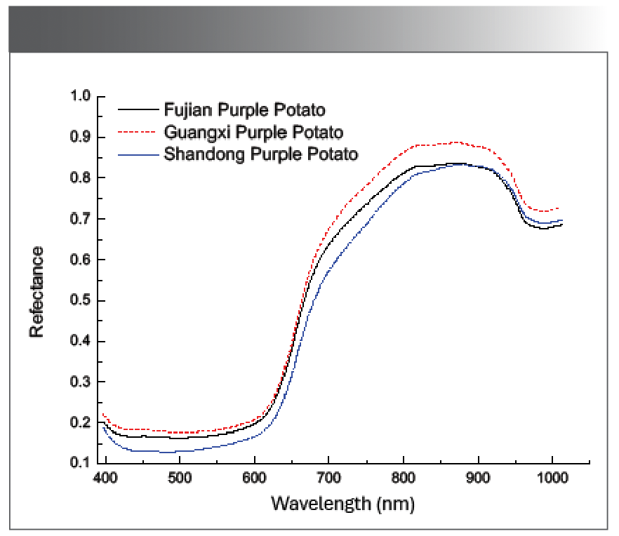
Figure 3 is the average reflection spectrum of purple sweet potatoes from three different geographic origins (Fujian, Guangxi, and Shandong). Its wavelength range is 400–1000 nm. It can be seen from Figure 3 that the trend of spectral changes of purple sweet potatoes from different origins is roughly the same. The spectral reflectance decreased first and then flattened. The lower reflectance in this band may be because of the presence of anthocyanins in the purple potato samples. The 610–820 nm band shows a monotonically increasing trend. The 820–920 nm band is a local strong reflection phenomenon, and the 920–1000 nm band shows a decreasing trend and tends to be gentle. The obvious absorption peak at 980 nm may be because of the change caused by the third-order frequency vibration of the O-H bond in water molecules. The spectral reflectance of purple potato in Guangxi is higher than that of Fujian purple potato and Shandong purple potato. The average spectrum of Guangxi purple potato and Shandong purple potato can be clearly distinguished. However, in the 630–680 nm band, the spectra of Guangxi purple potato and Fujian purple potato overlap, and in the range of 860–930 nm, Fujian purple potato and Shandong purple potato have overlapping parts. Therefore, the following will combine the chemometric method to process the reflection spectrum and establish mathematical models of different origins, so as to realize the identification of purple potatoes from different origins (27–29).

Figure 3: Average spectrum of purple sweet potatoes from different regions.

Variable Dimensionality Reduction and Feature Selection

Because of the huge amount of information contained in the hyperspectral data. The spectral variables contain useless information, and it is easy to reduce the model’s prediction accuracy during the modelling process. Therefore, to extract the effective information of the spectral variables to the greatest extent, this paper used PCA, SPA, and UVE to analyze and compare characteristic variables, thereby improving prediction accuracy and modelling efficiency of the purple sweet potato origin identification and detection model (30–33).

Dimensionality Reduction of Spectral Variables

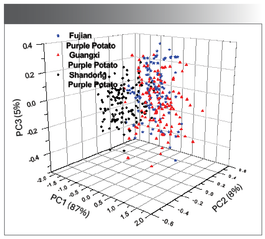
PCA is a method of reducing dimensions. The original variables are linearly transformed to obtain a small number of new variables. The new variables are used to characterize the data characteristics of the original variables. First, PCA was performed on the original spectra of purple sweet potatoes from different origins. PCA compressed spectral data was used to reduce the dimensions to obtain valid information representing the entire spectrum. We took the first three principal component scores to draw a spatial scatter plot of three samples from different origins. As shown in Figure 4, the first main component (PC1) contributed 86%, PC2 contributed 8%, PC3 contributed 5%, and the cumulative contribution reached 99%. It can be seen that the purple potato in Shandong has a good clustering phenomenon, and the purple potato in Fujian and the purple potato in Guangxi have mostly overlapped. The first three main components of PCA cannot distinguish the origin of purple sweet potatoes. Therefore, in this paper, the first 20 principal components are selected as input variables for subsequent models.

Figure 4: Scatter plot of the first three principal component scoring spaces.

Successive Projection Algorithm

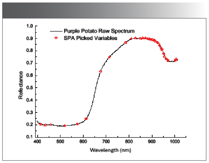
The successive projection algorithm (SPA) was used to screen the characteristic variables of the original spectral data. In the Matlab R2012a software, the maximum and minimum variables extracted in the SPA program were set to 60 and 10, respectively. The number of full-spectrum wavelength variables was 176, and 30 variables were screened out by SPA. Figure 5 is a graph of wavelength variables screened by the SPA algorithm. It can be seen from Figure 5 that in the 400–600 nm band, the selected variables are relatively gentle, and redundant information is effectively eliminated. The wavelengths of the selected variables are densely distributed between 800–1000 nm, and there are peaks and valleys in this band, which contains more effective information. Therefore, the selected 30 variables are used as input variables for subsequent models.

Figure 5: Wavelength variables screened by the SPA algorithm.

Elimination of No Information Variables

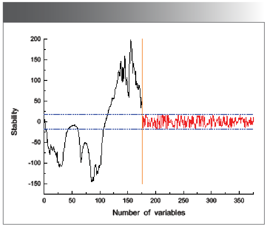
Wavelength variable screening was performed on the raw spectral data using uninformative variable elimination (UVE), as shown in Figure 6. The abscissa is the number of variables. There are 176 variables on the left of the orange vertical line as the original wavelength variables, and 200 on the right are the number of random variables set by the program. The ordinate is the stability value of the variable. The stability values corresponding to the two horizontal purple dotted lines are the thresholds of the screening wavelength variables, the spectral variables between the upper and lower thresholds are eliminated, and the spectral variables outside the upper and lower threshold intervals are retained. The wavelength variables selected by UVE are preferably 148 variables, which are used as input variables for subsequent modeling.

Figure 6: UVE algorithm wavelength variable screening.

Establishment and Prediction of Qualitative Discriminant Model of Purple Potato Origin

In this study, 40 purple potatoes from Guangxi, 40 purple potatoes from Fujian, and 40 purple potatoes from Shandong were selected. A total of 120 samples were collected for hyperspectral image acquisition. Three different positions in the middle of each image were used to extract the average spectrum. A total of 360 pieces of spectral data were used for model analysis. According to the Kennard-Stone algorithm, the number of samples is divided into 3:1, of which there are 273 correction sets (91 per origin) and 81 verification sets (29 per origin). Before establishing the model, the purple potato sample from Fujian was assigned a value of 1. The purple potato sample from Guangxi was assigned a value of 2, and the purple potato sample from Shandong was assigned a value of 3. The intermediate value of the two was taken as the classification threshold. If the predicted value is less than the threshold of 1.5, it is judged as Fujian purple potato; if the predicted value is between the threshold 1.5 and 2.5, it is judged as Guangxi purple potato; and if the predicted value is greater than the threshold of 2.5, it is judged as Shandong purple potato.

Study on the Partial Least Squares Discriminant Model of Purple Potato Origin Based on Spectral Characteristics

PCA, SPA, UVE, and other screening wavelength variables were used to screen the original spectrum. The variables obtained by the screening were used to establish a partial least squares discrimination (PLS-DA) model. Table I shows the PLS-DA model results of different variable selection methods. As can be seen from Table I, the modelling effect using the PCA, SPA, and UVE screening variables combined with the PLS-DA model is poor. As the number of variables in the input model increases, the better the modeling results may be, the use of the screening variable method may lead to removing valid information from the purple potato sample. The effect of modeling using raw spectral data is the best, where the root mean square error (RMSEC) of the modeling set is 0.273, the correlation coefficient (R_C) of the modeling set is 0.943, the total false positive rate is 6.591%, and the root mean square error of the prediction set is (RMSEP) is 0.357, the prediction set correlation coefficient (R_P) is 0.909, and the total false positive rate is 12.644%.

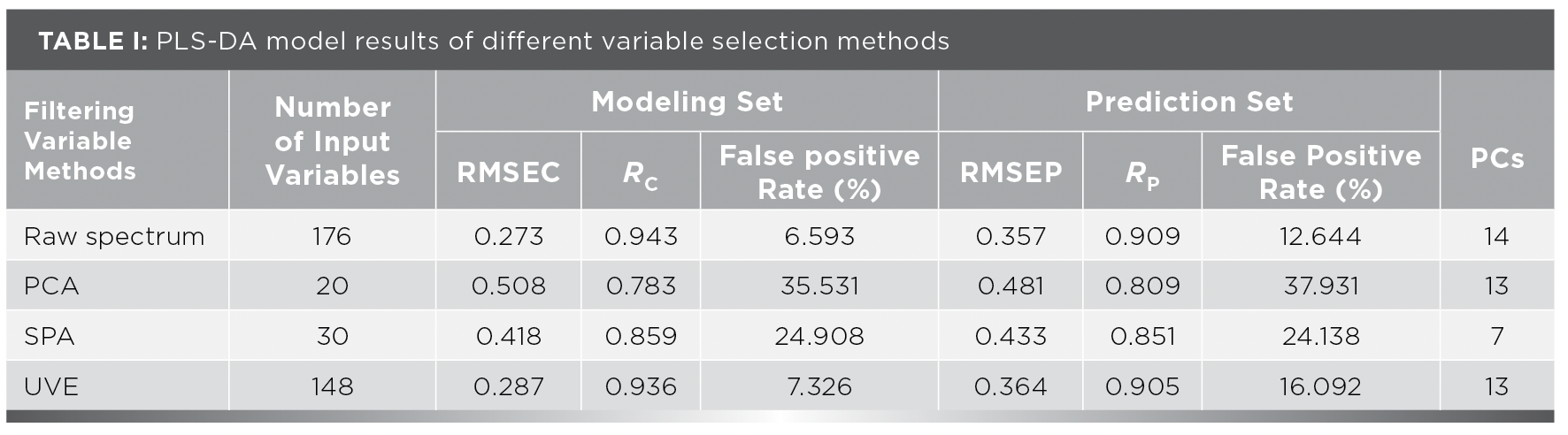
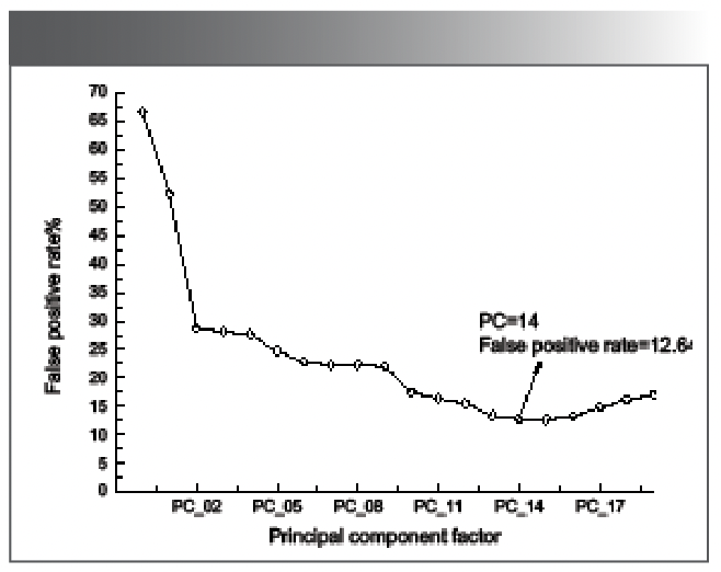
Selecting the appropriate principal component factor for modeling is the key to determining the performance of the PLS-DA model. If too few principal component (PCs) factors are selected in the modeling, the important information of the spectrum will be lost and the model accuracy will be reduced. Too many PCs will introduce more noise signals and affect model accuracy. The PLS-DA model uses the false positive rate to determine the optimal number of principal component factors. As shown in Figure 7, when the number of PC factors is 14, the total false positive rate of purple sweet potatoes is the lowest. Therefore, the optimal number of principal component factors is 14.

Figure 7: Optimal number of principal component factors.

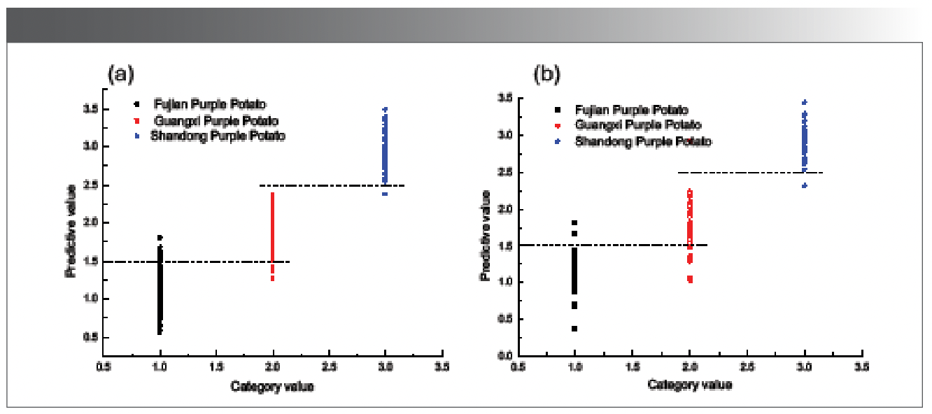
As shown in Figure 8, the partial least squares discriminant modelling set and prediction set classification diagram are shown. Figure 8 shows the number of misjudgments of the model set and prediction set of purple sweet potatoes from Fujian, Guangxi, and Shandong. In the modelling set, there are 91 spectra of purple sweet potatoes from each place of origin. The number of purple sweet potatoes in Fujian is 13, the number of purple sweet potatoes in Guangxi is 4, and the number of purple sweet potatoes in Shandong is 1. There are 29 spectra of purple potatoes from each place of origin in the prediction set, among which the number of misjudged purple Fujian potatoes is 2, the number of misjudged purple potatoes in Guangxi is 7, and the number of misjudged purple potatoes in Shandong is 2. The misjudgment rate of Shandong purple sweet potato is low. The total misjudgment rate of the modelling set is 6.591%, and the total misjudgment rate of the prediction set is 12.644%. The prediction ability of the model is relatively poor.

Figure 8: (a) Classification diagram of PLS-DA modeling set; (b) classification diagram of PLS-DA prediction set.

Study on the LS-SVM Discriminant Model of Purple Potato Origin Based on Spectral Features

The LS-SVM was used to discriminate the origin of purple sweet potatoes. LS-SVM is used to model two commonly used kernel functions: radial basis function (RBF-kernel) and linear function (LIN-kernel). There are two important parameters, γ (regularization parameter) and σ² (kernel parameter). The parameters affect the misjudgment rate of sample classification to a certain extent. The parameter is determined by a two-step search method. A large-step search is used to determine the boundary range of the nuclear parameters, and then small steps are used to search for the best parameters. The variables selected by PCA, SPA, UVE, and other methods are used as the model’s input variables. The prediction results of the LS-SVM model with different variable selection methods are shown in Table II.

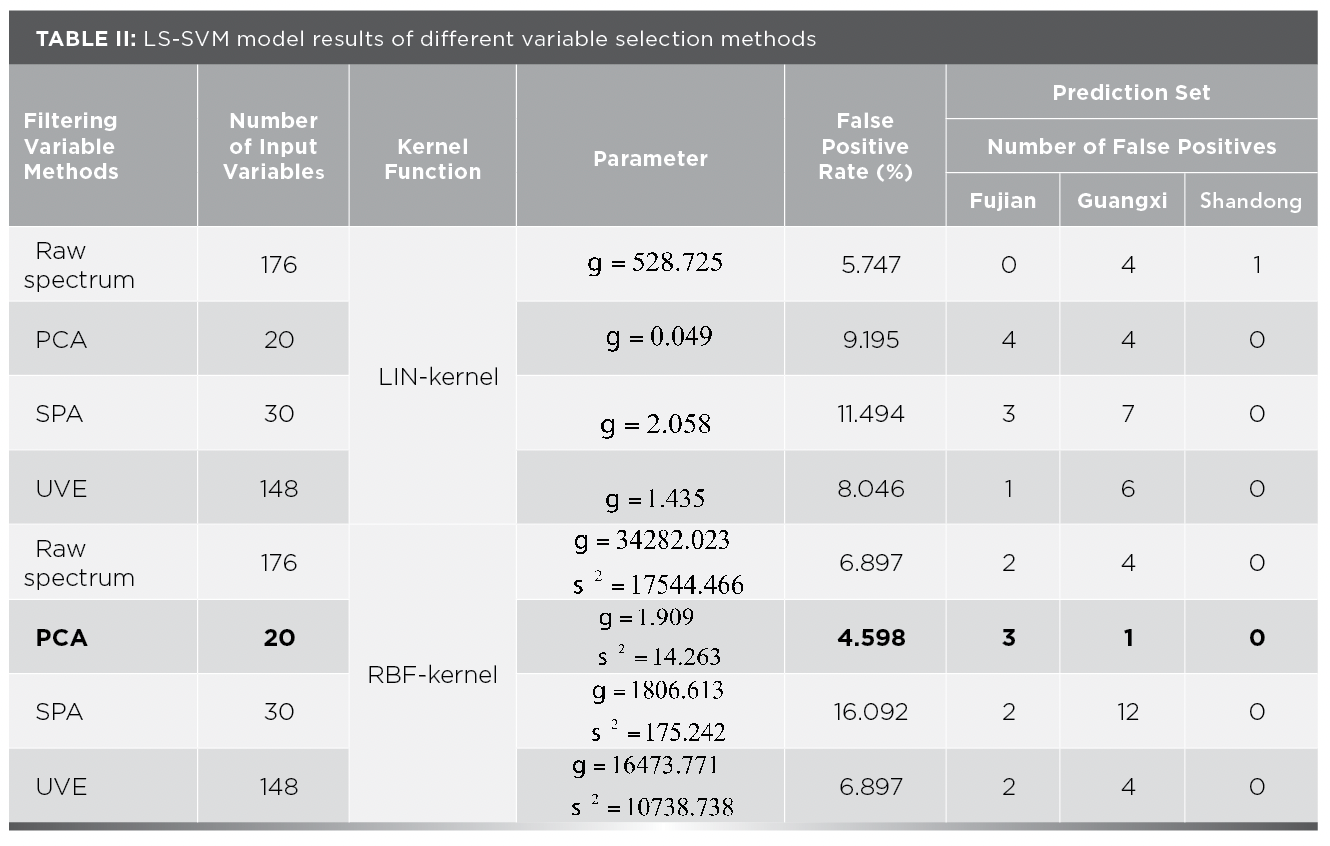
As can be seen from Table II, among the four different input variables using LIN-kernel, the LS-SVM model built using the original number of spectral variables has the lowest false positive rate, the false-negative rate is 5.747%, and its corresponding parameter γ is 528.725. The model established by the 30 variables screened by the SPA method had the highest false-positive rate, with a false positive rate of 11.494%. Among the four different input variables using RBF-kernel, the LS-SVM model built using the top 20 PC factors of PCA dimensionality reduction has the lowest false positive rate. The false-negative rate is as low as 4.598%, and its corresponding parameters γ, σ² is 1.909 and 14.263, respectively. Similarly, the model with the 30 variables selected by the SPA method has the highest false-positive rate, with a false positive rate of 16.092%. A comprehensive comparison shows that RBF is selected as the kernel function, and PCA is used as the dimensionality reduction method. The LS-SVM model established has the lowest false positive rate, indicating that the qualitative effect is the best.

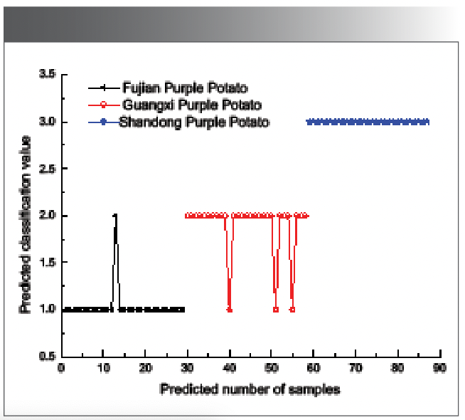
Figure 9 shows the classification of RBF-kernel in the top 20 PCs combined with LS-SVM. It can be seen from thefigure that 3 Fujian purple sweet potatoes were misjudged as Guangxi purple sweet potatoes, 1 Guangxi purple potato was misjudged as Shandong purple sweet potato, and Shandong purple sweet potato was 0. Therefore, the false positive rate is as low as 4.598%.

Figure 9: Classification chart of RBF-kernel function prediction set.

Study on the Discriminative Model of Purple Sweet Potato Origin Limit Learning Machine Based on Spectral Characteristics

An ELM is a feedforward neural network algorithm. Its feature is that the input weights and thresholds of hidden layer neurons are randomly generated, and only the number of hidden layer neurons needs to be constantly adjusted during the training process. The initial value of the number of hidden layer neurons is set to 10, and the step size is 10, which is sequentially increased to the number of samples in the modeling set, which is 273. The feature variables selected by different methods are used as inputs, and “sigmoidal”, “hardlim”, and “sine” are selected as the neuron excitation functions to establish the ELM prediction model. The optimal number of hidden layer neurons is determined by the accuracy of the classification. The statistical results of ELM prediction of different screening variables combined with different excitation functions are shown in Table III.

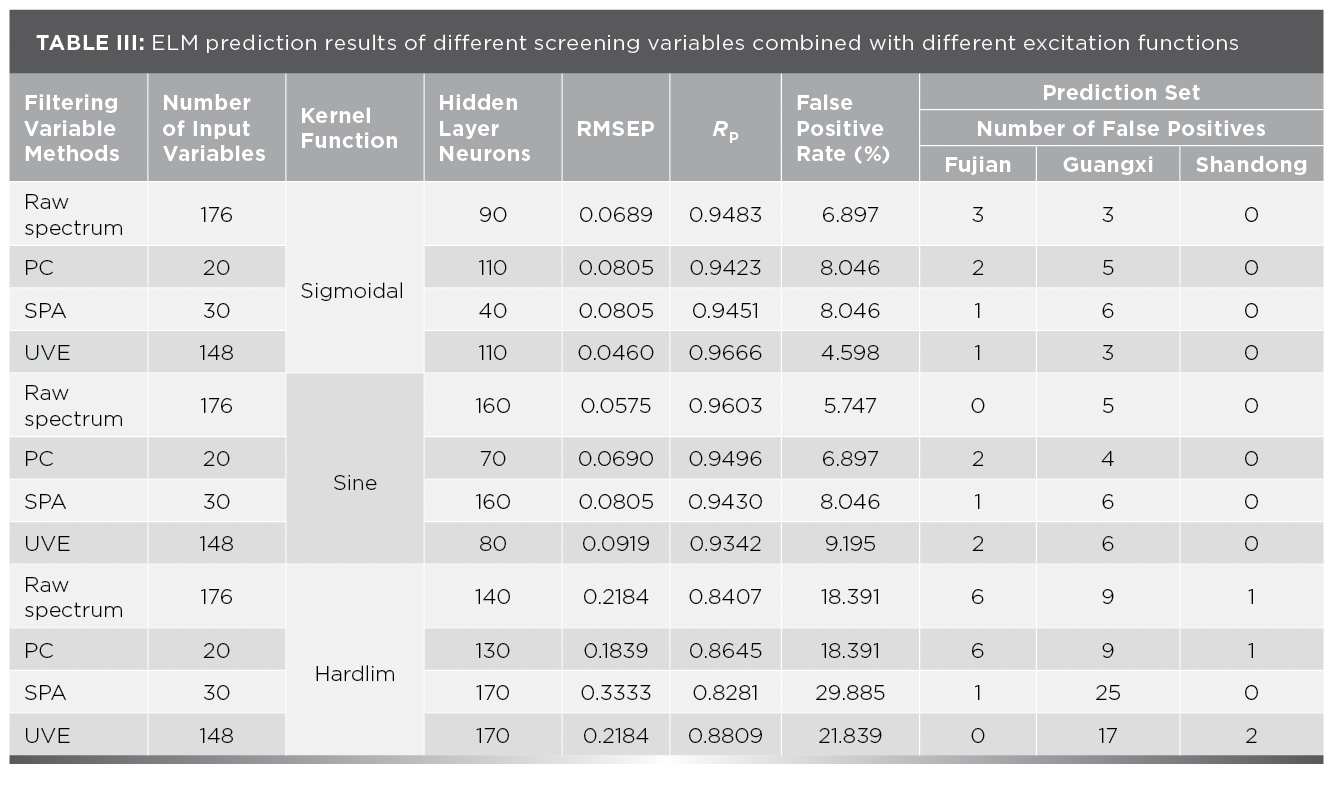
As can be seen from Table III, when the neuron excitation function is sigmoidal, the feature variable filtered by UVE and the number of hidden layer neurons is 110. The false positive rate of the ELM model is 4.598%. The prediction root mean square error is 0.0460, and the prediction correlation coefficient is 0.9666. When the neuron excitation function is sine, the original spectral data is used as input, and the number of hidden neurons is 160. The model’s false positive rate is 5.747%. The prediction root mean square error is 0.0575, and the prediction correlation coefficient is 0.9603. When the neuron excitation function is hardlim, the top 20 PC factors are used as inputs, and the number of hidden layer neurons is 130. The model’s false positive rate is 18.391%. The predicted root mean square error is 0.1839, and the predicted correlation coefficient is 0.8645. Compare the modeling results of different neuron excitation functions combined with different screening variables. Using the UVE screening variable method, the sigmoidal excitation function and the number of neurons in the hidden layer are 110, the modeling effect is the best.

To clearly compare the three kinds of characteristic variables and the original spectrum under which excitation function, the ELM model was used. The statistical results are shown in Table IV. As can be seen from Table V, the sigmoidal and sine two excitation functions combined with different characteristic variables are used to model a lower false positive rate. Both the PCA and SPA screening variable methods have decreased compared with the original spectrum, which may be due to the elimination of useful information by the screening variable method, resulting in poor model performance. Among them, the optimal screening variable method is UVE, which has a certain degree of improvement compared with the model established by the original spectrum, and its false positive rate has decreased by 1.149%, and the RMSEP has decreased by 0.0115.

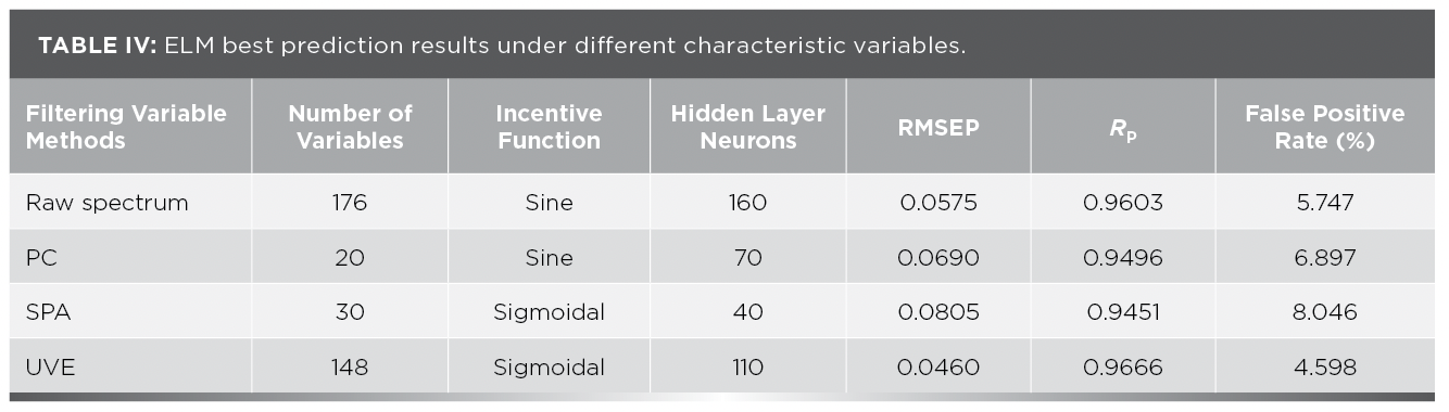
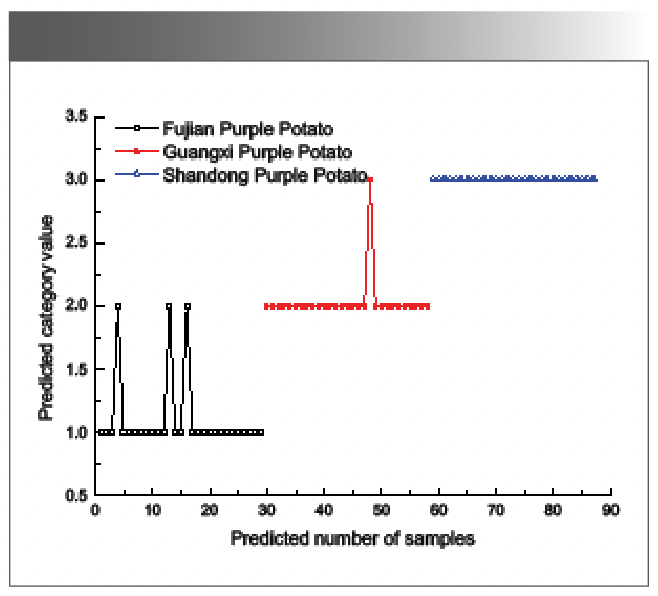
Figure 10 is a classification diagram of the ELM prediction set of the sigmoidal function of the UVE screening variables. It can be seen from Figure 10 that one Fujian purple potato was misjudged as Guangxi purple potato, three Guangxi purple potatoes were misjudged as Fujian purple potato, and Shandong purple potato was 0. The total false positive rate predicted by the ELM model is 4.598%.

Figure 10: Classification diagram of ELM prediction set for UVE screening variables.

Model Evaluation

An ELM is a feedforward neural network algorithm. Its feature is that the input weights and thresholds of hidden layer neurons are randomly generated. Only the number of hidden layer neurons needs to be constantly adjusted during the training process. The initial value of the number of hidden layer neurons is set to 10, and the step size is 10, which is sequentially increased to the number of samples in the modeling set, which is 273. The feature variables selected by different methods are used as inputs, and “sigmoidal,” “hardlim,” and “sine” are selected as the neuron excitation functions to establish the ELM prediction model. The accuracy of the classification determines the optimal number of hidden layer neurons. The statistical results of ELM prediction of different screening variables combined with different excitation functions are shown in Table III.

Conclusion

The geographical origin of the purple sweet potato is one of the most relevant factors that determine the quality and commercial value. The main objective of the current paper was to discriminate the different geographical origins of purple sweet potato rapidly using HSI. The differences among different geographical origins of purple sweet potato did exist in HSI. HSI combined with chemometric methods for discrimination of different geographical origins of purple sweet potato was a very attractive platform and had the potential to be widely used in rapid and on-site discrimination for its rapid, simple, and without any sample preparation.

Conflicts of Interest

The authors declare that there are no conflicts of interests regarding this research and publication of this manuscript.

Funding

The National Natural Science Foundation of China funded the research (No. 31760344), Science and Technology Research Project of Education Department of Jiangxi Province (Grant No. 190306). Science and Technology Research Project of Education Department of Jiangxi Province (Grant No. GJJ200652).

Author Contributions

Xiong Li conceived the study and performed the experiments. Yande Liu acquired the data. Yunjuan Yan edited the manuscript. Guantian Wang supervised every step of this research. All authors read and approved the manuscript.

References

1. Xu, M.; Li, J.; Yin, J. J.; et al. Color and Nutritional Analysis of Ten Different Purple Sweet Potato Varieties Cultivated in China via Principal Component Analysis and Cluster Analysis. Foods 2024, 13 (6). 904. DOI: 10.3390/foods13060904
2. Li, A.; Xiao, R.S.; He, S.; et al. Research Advances of Purple Sweet Potato Anthocyanins: Extraction, Identification, Stability, Bioactivity, Application, and Biotransformation. Molecules 2019, 24 (21), 13816. DOI: 10.3390/molecules24213816.
3. Yun, D.W.; Wu, Y.L; Yong, H.M; et al. Recent Advances in Purple Sweet Potato Anthocyanins: Extraction, Isolation, Functional Properties and Applications in Biopolymer-Based Smart Packaging. Foods 2024, 13 (21), 13485. DOI:10.3390/foods13213485.
4. Liu, W.; Liu, C. H.; Yu, J.; et al. Discrimination of Geographical Origin of Extra Virgin Olive Oils Using Terahertz Spectroscopy Combined with Chemometrics. Food Chem. 2018, 239, 81. DOI: 10.1016/j.foodchem.2018.01.081.
5. Sun, X.D.; Subedi, P.; Walker, R.; Walsh, K.B. NIRS Prediction of Dry Matter Content of Single Olive Fruit with Consideration of Variable Sorting for Normalisation Pre-treatment. Postharvest Bio. Technol. 2020, 166, 111140. DOI: 10.1016/j.postharvbio.2020.111140.
6. Liu, J.X.; Cao, Y.; Wang, Q.; et al. Rapid and Non-destructive Identification of Water-injected Beef Samples Using Multispectral Imaging Analysis. Food Chem. 2015, 188, 56. DOI: 10.1016/j.foodchem.2015.06.056.
7. Liu, W.; Liu, C.; Chen, F.; et al. Discrimination of Transgenic Soybean Seeds by Terahertz Spectroscopy. Sci. Rep. 2016, 6, 35799. DOI: 10.1038/srep35799.
8. Ma, S.Z.; Zhang, J.W.; Peng, M.J.; et al. Effects of Different Heat Treatment Methods on Physicochemical Characteristics and In Vitro Digestibility of Sweet Potato Flour and its Application in Meal Replacement Flour. J. Food Sci. 2024, 89 (10), 174481. DOI:10.1111/1750-3841.17481.
9. Steed, L. E.; Truong, V.-D. Anthocyanin Content, Antioxidant Activity, and Selected Physical Properties of Flowable Purple-Fleshed Sweetpotato Purees. J. Food Sci. 2008, 73 (5), E74. DOI: 10.1111/j.1750-3841.2008.00774.x.
10. Hao, Y.; Geng, P.; Wu, W. H.; et al. Identification of Rice Varieties and Transgenic Characteristics Based on Near-Infrared Diffuse Reflectance Spectroscopy and Chemometrics. Molecules 2019, 24 (24), 44568. DOI: 10.3390/molecules24244568.
11. Wei, L.; Hu, O.; Chen, H.; et al. Variety Identification and Age Prediction of Pu-erh Tea Using Graphene Oxide and Porphyrin Complex Based Mid-infrared Spectroscopy Coupled with Chemometrics. Microchem. J. 2020, 159, 105255. DOI:10.1016/j.microc.2020.105255.
12. Herzig, P.; Backhaus, A.; Seiffert, U.; et al. Genetic Dissection of Grain Elements Predicted by Hyperspectral Imaging Associated with Yield-related Traits in a Wild Barley NAM Population. Plant Sci. 2019, 284, 5. DOI: 10.1016/j.plantsci.2019.05.008.
13. Gao, Q. S.; Lim, S. S.; Jia, X. P. Spectral-Spatial Hyperspectral Image Classification Using a Multiscale Conservative Smoothing Scheme and Adaptive Sparse Representation. IEEE Trans. Geosci. Remote Sens. 2019, 57 (7), 4719–4732. DOI: 10.1109/TGRS.2019.2915809.
14. Fan, W. C.; Jiang, Y.; Huang, S. Y.; Liu, W. G. Research and Prediction of Opioid Crisis Based on BP Neural Network and Markov Chain. AIMS Mathematics 2019, 5 (1), 1357–1371. DOI: 10.3934/math.2019.5.1357.
15. Hu, Z.; Chen, Z.; Peng, B.; et al. Vehicle Lighting Recognition System Based on Erosion Algorithm and Effective Area Separation in 5G Vehicular Communication Networks. IEEE Access 2019, 7, 2927731. DOI: 10.1109/access.2019.2927731.
16. Baranowski, P.; Mazurak, W.; Pastuszka-Woźniak, J. Supervised Classification of Bruised Apples with Respect to the Time After Bruising on the Basis of Hyperspectral Imaging Data. Postharvest Biol. Technol. 2013, 86, 5. DOI: 10.1016/j.postharvbio.2013.07.005.
17. Huang, Y. F.; Dong, W. T.; Sanaei, A.; et al. Development of Simple Identification Models for Four Main Catechins and Caffeine in Fresh Green Tea Leaf Based on Visible and Near-infrared Spectroscopy. Computers and Electronics in Agric. 2020, 173, 105388. DOI: 10.1016/j.compag.2020.105388.
18. Devos, O.; Ruckebusch, C.; Durand, A.; et al. Support Vector Machines (SVM) in Near Infrared (NIR) Spectroscopy: Focus on Parameters Optimization and Model Interpretation. Chemom. Intell. Lab. Systems 2009, 95 (1), 11-005. DOI: 10.1016/j.chemolab.2008.11.005.
19. Liu, Q.; Tang, M.; Cai, J.; et al. Vis/NIR Hyperspectral Imaging for Detection of Hidden Bruises on Kiwifruits. Czech J. Food Sci. 2011, 69 (6), 532–539. DOI: 10.17221/69/2010-cjfs.
20. ElMasry, G.; Wang, N.; Vigneault, C.; Qiao, J.; ElSayed, A. Early Detection of Apple Bruises on Different Background Colors Using Hyperspectral Imaging. LWT - Food Sci. Technol. 2008, 41 (3), 309–317. DOI: 10.1016/j.lwt.2007.02.022.
21. Granato, D.; Santos, J. S.; Escher, G. B.; et al. Use of Principal Component Analysis (PCA) and Hierarchical Cluster analysis (HCA) for Multivariate Association Between Bioactive Compounds and Functional Properties in Foods: A Critical Perspective. Trends Food Sci. Technol. 2017, 70, 58–70. DOI: 10.1016/j.tifs.2017.12.006.
22. Liu, W.; Liu, C.H.; Yu, J. J.; et al. Discrimination of Geographical Origin of Extra Virgin Olive Oils Using Terahertz Spectroscopy Combined with Chemometrics. Food Chem. 2018, 239, 81. DOI: 10.1016/j.foodchem.2018.01.081.
23. Ramadan, Z.; Hopke, P. K.; Johnson, M. J.; Scow, K. M. Application of PLS and Back-Propagation Neural Networks for the Estimation of Soil Properties. Chemom. Intell. Lab. Systems 2005, 75 (1), 39–47. DOI: 10.1016/j.chemolab.2004.04.009.
24. Marrubini, G.; Papetti, A.; Genorini, E.; Ulrici, A. Determination of the Sugar Content in Commercial Plant Milks by Near Infrared Spectroscopy and Luff-Schoorl Total Glucose Titration. Food Anal. Methods 2016, 9 (11), 2977–2984. DOI: 10.1007/s12161-016-0713-1.
25. Ma, W. L.; Liu, H. A New Classification Method Based on the Deep Structure and Least Squares Support Vector Machine. Electronics Lett. 2020, 56 (10), 3776–3778. DOI: 10.1049/el.2019.3776.
26. Khalil, H. M.; El-Bardini, M. Implementation of Speed Controller for Rotary Hydraulic Motor Based on LS-SVM. Expert Sys. Appl. 2011, 38 (4), 4238–4244. DOI: 10.1016/j.eswa.2011.04.238.
27. Granato, D.; Koot, A.; van Ruth, S. M. Geographical Provenancing of Purple Grape Juices from Different Farming Systems by Proton Transfer Reaction Mass Spectrometry Using Supervised Statistical Techniques. J. Sci. Food Agric. 2015, 95 (13), 2668–2677. DOI: 10.1002/jsfa.7001.
28. Chiesa, L.; Panseri, S.; Bonacchi, S.; Procopio, A.; Zecconi, A.; Arioli, F.; Cuevas, F. J.; Moreno-Rojas, J. M. Authentication of Italian PDO Lard Using NIR Spectroscopy, Volatile Profile and Fatty Acid Composition Combined with Chemometrics. Food Chem. 2016, 5. DOI: 10.1016/j.foodchem.2016.05.180.
29. Müller-Maatsch, J.; Schweiggert, R. M.; Carlé, R. Adulteration of Anthocyanin- and Betalain-based Coloring Foodstuffs with the Textile Dye ‘Reactive Red 195’ and its detection by Spectrophotometric, Chromatic and HPLC-PDA-MS/MS Analyses. Food Cont. 2016, 6. DOI: 10.1016/j.foodcont.2016.06.012.
30. Liu, Y. D.; Cheng, M. J.; Hao, Y. Spectral Diagnostic Technology and its Application in Agricultural Product Quality Detection [J]. J. East China Jiaotong Univ. 2018, 35 (04): 1–7. DOI: 10.16749/j.cnki.jecjtu.2018.04.001
31. Li, B.; Su, C. T.; Yin, H.; Ou-Yang, A. G.; Liu, Y. D. High-spectral imaging combined with curvature-assisted Hough transformation circle detection and improved Otsu detection of bruised peaches. J. Food Measure Characterization 2024, 8 (3), 2541–2547. DOI: 10.1007/s11694-024-02541-7.
32. Nunes, C. A.; Alvarenga, V. O.; Sant’Ana, A. d. S.; Santos, J. S.; Granato, D. The Use of Statistical Software in Food Science and Technology: Advantages, Limitations, and Misuses. Food Res. Int. 2015, 73, 66–74. DOI: 10.1016/j.foodres.2015.06.011.
33. Walsh, K. B.; Blasco, J.; Zude-Sasse, M.; Sun, X. Visible-NIR ‘Point’ Spectroscopy in Postharvest Fruit and Vegetable Assessment: The Science Behind Three Decades of Commercial Use. Postharvest Biol. Technol. 2020, 6. DOI: 10.1016/j.postharvbio.2020.111246.

Xiong Li, Yande Liu, Yunjuan Yan, and Guantian Wang are with the School of Mechatronics and Vehicle Engineering at East China Jiaotong University, in Nanchang, China.Li, Liu, and Wang are also with the Institute of Intelligent Mechanical and Electrical Equipment Innovation at East China Jiaotong University, in Nanchang, China. Direct correspondence to Yande Liu at jxliuyd@163.com ●