Stable Variable Selection Method and Comparison for Quantitative Analysis of Steels Using Laser-Induced Breakdown Spectroscopy

In this work, a stable variable selection method based on variable stability correction (VSC) and modified iterative predictor weighting-partial least squares (mIPW-PLS) is proposed for the quantitative analysis of steel samples by laser-induced breakdown spectroscopy (LIBS). This method takes stability as the variable selection criterion, which has strong adaptability to the quantitative analysis of different sample partitions of the steel data set. To demonstrate the feasibility and effectiveness of the proposed method, we compared the successive projections algorithm (SPA) and uninformative variable elimination (UVE) to detect nine sample partitions of different elements in steel. The experimental results showed that the VSC-mIPW-PLS algorithm could achieve credible quantitative analysis accuracy for nine sample partitions of three elements. The root mean square errors of prediction (RMSEP) were no more than 5.1817 (chromium), 1.9759 (nickel), and 2.5848 (manganese), which proved credible prediction ability. This method has the potential for applications using LIBS spectrometers for industrial field and research experiments.

Steel is the primary raw material of heavy industry. Added elements play a crucial role in the properties of steel products during their smelting process (1,2). Currently, steel analysis techniques, such as inductively coupled plasma–atomic emission spectrometry (ICP-AES), (3) flame atomic absorption spectrometry (FAAS), (4) hydride generation–atomic absorption spectrometry, (5) and hydride generation–atomic fluorescence spectrometry (6) have been put into use in the steel industry. However, these methods can obtain high-precision detection results, and sample preparation and sample digestion are time-consuming and complex.Therefore, traditional detection methods still need to meet the need for rapid detection. Laser-induced breakdown spectroscopy (LIBS) is an atomic emission spectroscopy technique with simple sample preparation and real-time detection advantages. It has shown its application potential in many fields, such as quantitative analysis of soil (7,8), heavy metals (9), and coal (10). Chemometric methods have been used by researchers to do a large amount of spectral pretreatment (11), abnormal sample removal, multivariate correction, pattern recognition (12,13), and feature wavelength selection for LIBS data (14). Among them, variable selection is of great concern. With the improvements of measurement technology, the high resolution and wide detection range of spectrometers can obtain high-dimensional data, which is likely conducive to the application of multivariate analysis. Many studies prove that multivariate analysis models are more robust and accurate than univariate analysis (15). However, with the increase in the number of samples, the data contains more noise and useless information. Calculating the multivariate model established using the original full-spectrum data is complex and time-consuming. Noise and useless information affects the accuracy and stability of the model, and the multicollinearity between variables also affects the modeling, which is important for research and practical applications. Therefore, variable selection has become an indispensable step in multivariate model construction. Various methods of variable selection have been reported in many papers. Massart et al proposed an uninformative variable elimination (UVE) method to calculate the stability of each variable by adding random noise to the data, which is used to remove uninformative variables (16). The interval partial least squares (iPLS) method was proposed by Norgaard et al. iPLS divides the spectrum into several consecutive subintervals of equal width (17). The partial least squares (PLS) model was established for each sub-interval, and the optimal model band was determined according to the root mean squared error of cross-validation (RMSECV). Wold et al. proposed the variable importance projection (VIP) method (18). In VIP analysis, variables convey their explanatory power to target values through principal components. Forina et al proposed iterative predictor weighting (IPW), a cyclic iteration method based on PLS regression, to eliminate useless predictors in multiple regression problems (19). Araújo et al. developed the successive projections algorithm (SPA) as a forward feature variable selection method (20).

The variable selection method was initially proposed for near-infrared spectroscopy rather than LIBS applications. The reason may be that the near-infrared band is dominated by the molecular spectrum (band spectrum), while LIBS is dominated by the atomic spectrum (line spectrum). At present, many researchers apply these classical variable selection methods in LIBS. Pontes et al. adopted SPA, GA, and other algorithms for variable selection and used data compression programs in the wavelet domain to reduce the computational workload without significantly affecting the results (21). In our earlier work, we presented an automatic variable selection method for laser-induced breakdown spectra (LIBS) based on full spectrum correction (FSC) and modified iterative predictor weighting-partial least squares (mIPW-PLS) (22). It is noteworthy that researchers usually divide the data set into a training set and a test set in a particular proportion before variable selection. Then they use the training set to generate the model and then use the test set to test the model and verify its validity (23). Nevertheless, the final evaluation measures calculated on the test set have a strong relationship with the original partition, and the results can change under different partitions (24). In other words, the existing variable selection methods have poor robustness to the results calculated by partitioning different data sets, so finding a sample partition with a better evaluation index is inevitable.

This paper proposes a stable variable selection method applied to LIBS technology, which uses a more informative criterion to select essential variables, namely variable stability. It is adaptable to quantitative analysis of different partitions of steel data sets and eliminates manual processes. To demonstrate the superiority and feasibility of this method, we compared the quantization results with the traditional algorithms of SPA and UVE under different partitions. Stability is defined as the absolute value of a variable divided by its standard deviation.

Theory and Method

Modified Iterative Predictor Weighing- Partial Least Squares (mIPW-PLS)

IPW-PLS is a method used to eliminate unwanted predictors in multiple regression problems. The method is based on cyclic repetition of PLS regression (25); in each loop, the importance of the variable is calculated and multiplied by the variable itself. The importance of a variable is defined as (19):

where s_j and b_j are the standard deviations and PLS regression coefficient of the corresponding variable j, and n is the number of variables in the current cycle. The problematic threshold of the current IPW period is calculated as (26):

where σ is the standard deviation of all variables included in the current period, and n is the number of variables in the current period. Furthermore, delete the corresponding variable j, whose importance is less than Thr.

Variable Stability Factor

To carry out variable selection effectively while maintaining high accuracy and robustness in this work, we developed an automatic variable selection method based on variable stability based on previous research. The new method adopts a defined variable stability factor, which is defined as:

Where c_j is corresponding to the stability factor of the variable j, (d_j) is the jth column of the average of the spectral matrix X. s(dj) is the jth column standard deviation of spectrum matrix X, and all variables are multiplied by the vector C = [c₁,c₂…,c_n]. The variable stability factor is used to overcome the problem that the traditional algorithm has poor adaptability to the quantitative analysis of different data set partitions.

Stable Variable Selection Method Based on Variable Stability Correction and mIPW-PLS (VSC-mIPW-PLS)

In terms of the large amount of spectral data in the LIBS experiment and the poor adaptability of the traditional algorithm to the quantitative analysis of different data set partitions, this paper proposes a stable variable selection method based on improving previous studies. The new method uses the defined variable stability factor combined with mIPW-PLS to realize automatic selection. The specific selection functions and procedures are shown in Figure 1.

FIGURE 1: The process and functions of VSC-mIPW-PLS.

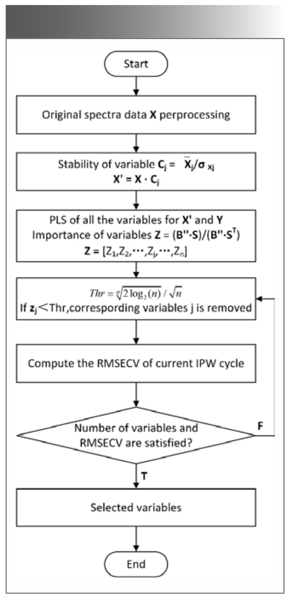
The whole method can be broken down into several steps:

1. Perform normalization, wavelet denoising, and other spectral data preprocessing to improve spectral quality.

2. Calculate the stability of all variables by multiplying the variables by the corresponding stability factor.

3. Calculate PLS regressions for all variables, as well as the importance Z of the variable.

4. Calculate the hard threshold Thr of the current IPW period is calculated according to equation 2. If any significance z_j is less than Thr, the corresponding variable j is removed.

5. Use the number of remaining variables and the root mean square error (RMSECV) of cross-validation to determine whether to stop the IPW cycle or return to step (4).

In this work, the programs of the method were written in Matlab (version 2021b, MathWorks).

Experimental

Samples

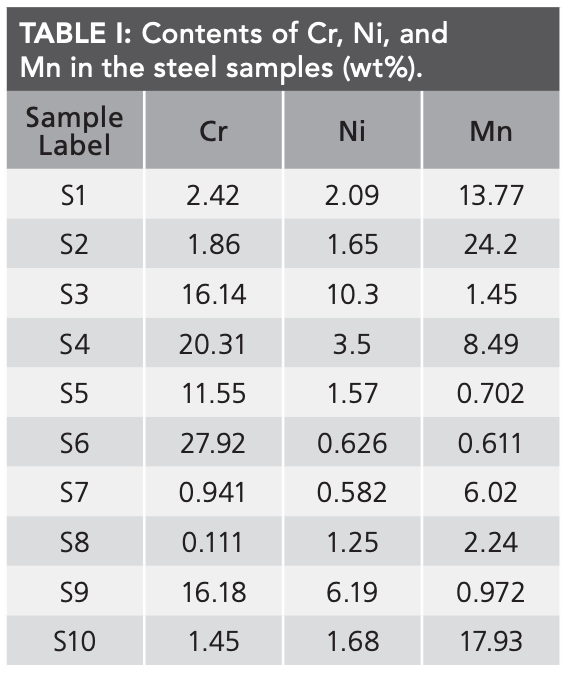
This study analyzed 10 different steel samples and labeled S1-S10: YSBS37354-18-S1, YSBS37355-18-S2, YSBS37361-10-S3, YSBS37373-14-S4, YSBS37077-15-S5, YSBS37098-15-S6, YSBS37346-13-S7, YSBS37036-16-S8, YSBS37393-16-S9, YSBS37343-13-S10. All steels are certified as reference materials by the Shanghai research Institute of Materials (SRIM). Five individual spectra were collected from different locations of each sample and averaged to avoid variable composition of the steel samples. Each sample is a Φ32×24 cylinder. The metal concentration in the sample is shown in Table I. The above samples were randomly divided, and nine different partitioning conditions were obtained, labeled SP1-SP9. The specific partitioning conditions are shown in Table II. The proportion of the training and test sets in each partitioning was the same.

Instrumentation

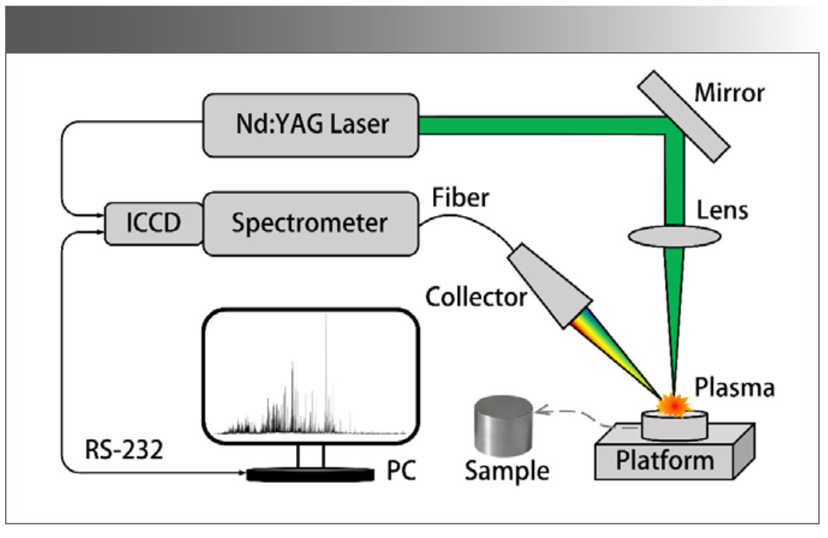
The LIBS system device used in this experiment is shown in Figure 2. A Q-switched Nd: YAG laser (EKSPLA, NT352C-20-FWS) was used as the light source to generate laser excitation samples with a wavelength of 1064 nm, a laser repetition rate of 20 Hz, pulse duration of > 5 μs, a pulse rise time of 50 ns, and pulse jitter of ±0.5 ns. The delay value between the lamp flash and Q-switch pulse equals 270 μs. The energy per pulse is 300 mJ. The laser beam passes through a reflecting prism and a focusing lens (f = 75 mm) and is focused 1 mm below the sample’s surface. Spectra were collected by an achromatic concentrator and analyzed by fiber coupling to a mid-step spectrometer (LTB, ARYELLE 200). The ICCD camera of the spectrometer and Nd:YAG laser is combined with the computer for synchronous signal transmission. The ICCD works in sync with the external trigger signal of the laser device. We first cleaned the steel sample’s surface with a laser to avoid contamination in the experiment. Furthermore, we accumulated 20 laser pulses from each point into an original spectrum to ensure the stability of the spectrum.

FIGURE 2: Schematic of the LIBS experimental setup.

Results and Discussion

Due to the matrix effect, laser pulse fluctuation, ambient temperature, and other external factors, the spectrum of each steel sample will be seriously disturbed. Therefore, it is indispensable to preprocess the original spectrum to eliminate the interference existing in the whole spectrum. This work first uses wavelet transform to smooth the spectrum denoising to eliminate noise interference. Then the mean normalization of the denoised spectrum is carried out to correct the differences caused by external factors in these spectra. Different wavelet functions and a different number of decomposition layers will impact the results differently. This paper combines different wavelet functions and decomposition layers to process the original spectrum for optimal preprocessing results. It can be seen in Figure 3 that the highest signal-to-noise ratio can be obtained by using the wavelet function sym10 and the number of decomposition layers of one layer.

FIGURE 3: Determination of wavelet function and decomposition level.

Sample Partition

This paper separately studied the model established by SPA and UVE under nine different sample partitions and compared the results to prove the algorithm’s feasibility. UVE is repeated five times to obtain the optimal solution because the added random noise will cause the results to be inconsistent every time. RMSECV determines the optimal parameters (the number of folds of cross-validation) set via SPA. Cr, Ni, and Mn variables are 32, 28, and 25, respectively. The number of IPW cycles is determined by considering RMSECV and the number of variables.

The results of VSC-mIPW-PLS selection of three metal elements for SP1 are shown in Figure 4. Figure 5 shows the relationship between RMSEP and sample partitioning under three different algorithms for the Cr element. RMSEP can be used to measure the difference between the predicted value and the actual value, reflect the degree of deviation between the predicted value and the actual value, evaluate the accuracy of the model. The smaller the RMSEP, the more stable the predictive model.

FIGURE 4: Variables selected by VSC-mIPW-PLS for Cr, Ni, and Mn elements.

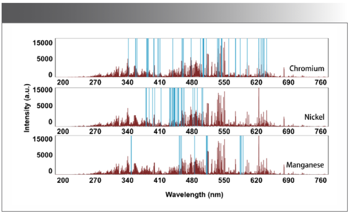
FIGURE 5: RMSEP for Cr in different sample partitions.

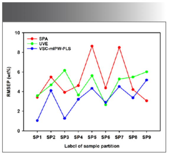
The results show that VSC-mIPW-PLS can obtain smaller RMSEP for different sample partitions, which reflects credible predictive ability. It is worth noting that the algorithm achieves very small RMSEP under SP1 and SP3 partitions, and the RMSEP of other partitions is also comparable to the partition of better results in SPA and UVE. In addition, other partitions’ results fluctuate in a small range and have high stability except for SP1 and SP3. Figure 6 shows the result of element Ni. RMSEP obtained by this algorithm is very small for these nine different sample partitions, demonstrating satisfactory quantification accuracy.

FIGURE 6: RMSEP for Ni in different sample partitions.

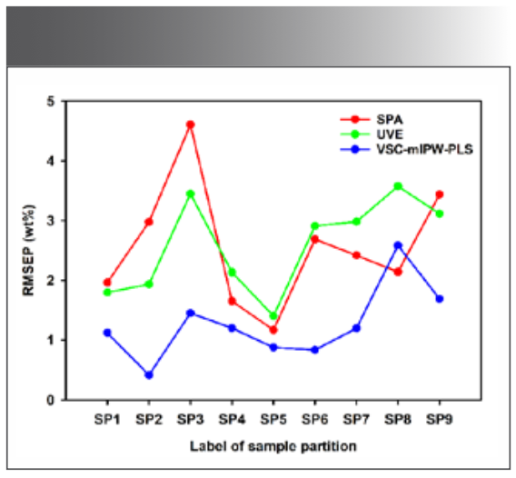
It is also worth noting that VSC-mIPW-PLS shows better stability with large fluctuations of traditional algorithm results in the partition, such as SP5-SP8. The results of the Mn element are shown in Figure 7. The results obtained by VSC-mIPW-PLS in other partitions are stable, and RMSEP is negligible except for SP8. VSC-mIPW-PLS has strong adaptability to quantitative analysis of different partitions of data sets. As described in the introduction, this method eliminates manual processes and saves much time for researchers.

FIGURE 7: RMSEP for Mn in different sample partitions.

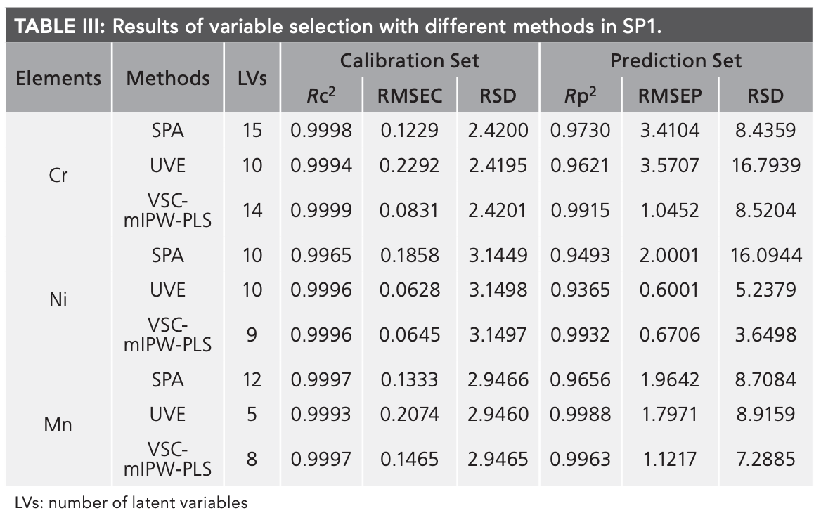
For Cr, Ni, and Mn, SP1 was the partition that the three variable selection methods obtained satisfactory quantitative analysis. Detailed results are shown in Table III. It can be seen from the table that the three methods can all achieve sound prediction effects, which means that the result of VSC-mIPW-PLS is equivalent to the result of SPA and UVE. The RSDs of the verification and prediction sets reflects that VSC-mIPW-PLS have better accuracy in analyzing test results. RSDs can analyze the precision of the results in the inspection and inspection work The smaller the RSD value, the higher the precision of the model. For UVE, the added random noise matrix may be the main factor to reduce the accuracy of the results.

Quantitative Analysis

In this study, variables selected by UVE, SPA, and VSC-mIPW-PLS were used to model the quantitative analysis of the LIBS experiment based on the PLS model. Test sets are used to verify the predictive performance of the model. Figure 8 shows the overall effect of quantitative analysis. The four subgraphs in each row show the models from left to right using the original spectrum, SPA, UVE, and VSC-mIPW-PLS. In each column, the three subgraphs show each metal element (chromium, nickel, and manganese) from top to bottom using the same algorithm. The key indexes in the model are the number of selection variables, root mean square error correction (RMSEC), and root mean square error prediction (RMSEP).

FIGURE 8: Quantification results with different methods for different elements: (a) PLS for Cr, (b) SPA for Cr, (c) UVE for Cr, (d) VSC-mIPW-PLS for Cr, (e) PLS for Ni, (f) SPA for Ni, (g) UVE for Ni, (h) VSC-mIPW-PLS for Ni, (i) PLS for Mn, (j) SPA for Mn, (k) UVE for Mn, (l) VSC-mIPW-PLS for Mn.

Some conclusions can be drawn from these figures. The RMSEC and RMSEP values of the three optimization models are better than those of the PLS model. The variable selection method is an effective means to improve the quantitative analysis results. Nevertheless, due to the high concentration of Mn, the spectral line is relatively less interfered with, so the improvement effect could be more evident in the case of Mn. The quantitative precision of different elements is also different for the three variable selection methods, among which UVE is slightly dominant. It is worth noting that VSC-mIPW-PLS, as a stable variable selection method, achieved more satisfactory performance in SP1, where the three methods obtained good results. The RMSEP of the VSC-mIPW-PLS model for Ni is better than SPA, and RMSEP for Mn is better than UVE, reflecting satisfactory quantitative accuracy.

Conclusions

This paper proposes a stable variable selection method applied to LIBS technology, which applies a more informative criterion, namely variable stability, to select important variables. Stability is defined as the absolute value of a variable divided by its standard deviation, which eliminates the manual process and saves researchers time. The method is compared with the traditional method. The experimental results show that SPA, UVE, and VSC-mIPW-PLS can effectively select variables. For different data set partitions, VSC-mIPW-PLS showed stable and satisfactory quantitative accuracy. The RMSEPs of the SP9 model with the worst prediction ability were 5.1817 (chromium), 0.2407 (nickel), and 1.6885 (manganese), respectively. The results are comparable to the best partitioning of UVE and SPA. VSC-mIPW-PLS achieved more satisfactory performance than traditional methods in SP1, where the three variable selection methods obtained good results. This study provides a stable variable selection method for the variable selection of LIBS technology, which has strong adaptability to the quantitative analysis of different partitions of data sets.

Author Information

The authors declare no competing financial interest.

Acknowledgments

This work was supported in part by National key research and development plan project (2020YFB2010800), National Natural Science Foundations of China under Grant (61971307,61905175), State Key Laboratory Exploratory Project (Pilt2103), the Fok Ying Tung education foundation (171055), Young Elite Scientists Sponsorship Program by CAST (2021QNRC001), Guangdong Province key research and development plan project (2020B0404030001), National Defense Science and Technology Key Laboratory Fund (6142212210304).

References

(1) Lau, S. K.; Cheung, N. H. Minimally Destructive and Multi-Element Analysis of Steel Alloys by Argon Fluoride Laser-Induced Plume Emissions. Appl. Spectrosc. 2009, 63 (7), 835–838. DOI: 10.1366/000370209788700973

(2) Li, J. M.; Xu, M. L.; Ma, Q. X.; Zhao, N.; Li, X. Y.; Zhang, Q. M.; Guo, L.; Lu, Y. F. Sensitive Determination of Silicon Contents in Low-Alloy Steels Using Micro Laser-Induced Breakdown Spectroscopy Assisted with Laser-Induced Fluorescence. Talanta 2019, 194, 697–702. DOI: 10.1016/j.talanta.2018.10.069

(3) Adya, V. C.; Sengupta, A.; Thulasidas, S. K.; Natarajan, V. Direct Determination of S and P at Trace Level in Stainless Steel by CCD-based ICP-AES and EDXRF: A Comparative Study. Atom. Spectrosc. 2016, 37 (1), 19–24. DOI: 10.46770/as.2016.01.004

(4) Yebra-Biurrun, M. C. Flame Atomic Absorption Determination of Trace Cobalt in Steel Samples Using a Flow-Injection On-Line Separation System. Lab. Robot. Autom. 1998, 10 (5), 299–305. DOI: 10.1002/(SICI)1098-2728(1998)10:5%3C299::AID-LRA6%3E3.0.CO;2-%23

(5) Klassen, A.; Kim, M. L.; Tudino, M. B.; Baccan, N.; Arruda, M. A. Z. A Metallic Furnace Atomizer in Hydride Generation Atomic Absorption Spectrometry: Determination of Bismuth and Selenium. Spectroc. Acta Pt. B–Atom. Spectr. 2008, 63 (8), 850–855. DOI: 10.1016/j.sab.2008.03.012

(6) Chen, L. C.; Yang, F. M.; Xu, J.; Hu, Y.; Hu, Q. H.; Zhang, Y. L.; Pan, G. X. Determination of Selenium Concentration of Rice in China and Effect of Fertilization of Selenite and Selenate on Selenium Content of Rice. J. Agric. Food Chem. 2002, 50 (18), 5128–5130. DOI: 10.1021/jf0201374

(7) Fu, X.; Duan, F. J.; Huang, T. T.; Ma, L.; Jiang, J. J.; Li, Y. C. A Fast Variable Selection Method for Quantitative Analysis of Soils Using Laser-Induced Breakdown Spectroscopy. J. Anal. At. Spectrom. 2017, 32 (6), 1166–1176. DOI: 10.1039/c7ja00114b

(8) Bousquet, B.; Sirven, J. B.; Canioni, L. Towards Quantitative Laser-Induced Breakdown Spectroscopy Analysis of Soil Samples. Spectroc. Acta Pt. B–Atom. Spectr. 2007, 62 (12), 1582–1589. DOI: 10.1016/j.sab.2007.10.018

(9) Yang, L.; Meng, L. W.; Gao, H. Q.; Wang, J. Y.; Zhao, C.; Guo, M. M.; He, Y.; Huang, L. X. Building a Stable and Accurate Model for Heavy Metal Detection in Mulberry Leaves Based on a Proposed Analysis Framework and Laser-Induced Breakdown Spectroscopy. Food Chem. 2021, 338, 9. DOI: 10.1016/j.foodchem.2020.127886

(10) Yao, S. C.; Mo, J. H.; Zhao, J. B.; Li, Y. S.; Zhang, X.; Lu, W. Y.; Lu, Z. M. Development of a Rapid Coal Analyzer Using Laser-Induced Breakdown Spectroscopy (LIBS). Appl. Spectrosc. 2018, 72 (8), 1225–1233. DOI: 10.1177/0003702818772856

(11) Wang, L. S.; Yang, X. Y.; Xi, S. F.; Mo, J. Y. Wavelet Smoothing and Denoising to Process Capillary Electrophoresis Signals. Chem. J. Chin. Univ.-Chin. 1999, 20 (3), 383–386.

(12) Li, Q. B.; Gao, Q. S.; Zhang, G. J. Improved Extended Multiplicative Scatter Correction Algorithm Applied in Blood Glucose Noninvasive Measurement with FT-IR Spectroscopy. J. Spectrosc. 2013, 2013, 5. DOI: 10.1155/2013/916351

(13) Windig, W.; Shaver, J.; Bro, R. Loopy MSC: A Simple Way to Improve Multiplicative Scatter Correction. Appl. Spectrosc. 2008, 62 (10), 1153–1159. DOI: 10.1366/000370208786049097

(14) Maugis, C.; Celeux, G.; Martin-Magniette, M. L. Variable Selection in Model-Based Clustering: A General Variable Role Modeling. Comput. Stat. Data Anal. 2009, 53 (11), 3872–3882. DOI: 10.1016/j.csda.2009.04.013

(15) Yeh, C. T. Reduction to Least-Squares Estimates in Multiple Fuzzy Regression Analysis. IEEE Trans. Fuzzy Syst. 2009, 17 (4), 935–948. DOI: 10.1109/tfuzz.2008.926588

(16) Centner, V.; Massart, D. L.; de Noord, O. E.; de Jong, S.; Vandeginste, B. M.; Sterna, C. Elimination of Uninformative Variables for Multivariate Calibration. Anal. Chem. 1996, 68 (21), 3851–3858. DOI: 10.1021/ac960321m

(17) Norgaard, L.; Saudland, A.; Wagner, J.; Nielsen, J. P.; Munck, L.; Engelsen, S. B. Interval Partial Least-Squares Regression (iPLS): A Comparative Chemometric Study with An Example From Near-Infrared Spectroscopy. Appl. Spectrosc. 2000, 54 (3), 413–419. DOI: 10.1366/0003702001949500

(18) Farres, M.; Platikanov, S.; Tsakovski, S.; Tauler, R. Comparison of the Variable Importance in Projection (VIP) and of the Selectivity Ratio (SR) Methods for Variable Selection and Interpretation. J. Chemometr. 2015, 29 (10), 528–536. DOI: 10.1002/cem.2736

(19) Forina, M.; Casolino, C.; Millan, C. P. Iterative Predictor Weighting (IPW) PLS: A Technique for the Elimination of Useless Predictors in Regression Problems. J. Chemometr. 1999, 13 (2), 165–184.

(20) Araujo, M. C. U.; Saldanha, T. C. B.; Galvao, R. K. H.; Yoneyama, T.; Chame, H. C.; Visani, V. The Successive Projections Algorithm for Variable Selection in Spectroscopic Multicomponent Analysis. Chemometrics Intell. Lab. Syst. 2001, 57 (2), 65–73. DOI: 10.1016/s0169-7439(01)00119-8

(21) Pontes, M. J. C.; Cortez, J.; Galvao, R. K. H.; Pasquini, C.; Araujo, M. C. U.; Coelho, R. M.; Chiba, M. K.; de Abreu, M. F.; Madari, B. E. Classification of Brazilian Soils by Using LIBS and Variable Selection in the Wavelet Domain. Anal. Chim. Acta 2009, 642 (1–2), 12–18. DOI: 10.1016/j.aca.2009.03.001

(22) Duan, F. J.; Fu, X.; Jiang, J. J.; Huang, T. T.; Ma, L.; Zhang, C. Automatic Variable Selection Method and a Comparison for Quantitative Analysis in Laser-Induced Breakdown Spectroscopy. Spectroc. Acta Pt. B–Atom. Spectr. 2018, 143, 12–17. DOI: 10.1016/j.sab.2018.02.010

(23) Mahmud, M. S.; Huang, J. Z.; Salloum, S.; Emara, T. Z.; Sadatdiynov, K. A Survey of Data Partitioning and Sampling Methods to Support Big Data Analysis. Big Data Min. Anal. 2020, 3 (2), 85–101. DOI: 10.26599/bdma.2019.9020015

(24) Zhan, X. R.; Zhu, X. R.; Shi, X. Y.; Zhang, Z. Y.; Qiao, Y. J. Determination of Hesperidin in Tangerine Leaf by Near-Infrared Spectroscopy with SPXY Algorithm for Sample Subset Partitioning and Monte Carlo Cross Validation. Spectrosc. Spectr. Anal. 2009, 29 (4), 964–968. DOI: 10.3964/j.issn.1000-0593(2009)04-0964-05

(25) Wold, S.; Sjostrom, M.; Eriksson, L. PLS-Regression: A Basic Tool of Chemometrics. Chemometrics Intell. Lab. Syst. 2001, 58 (2), 109–130. DOI: 10.1016/s0169-7439(01)00155-1

(26) Chen, D.; Hu, X. G.; Shao, X. G.; Su, Q. D. Variable Selection by Modified IPW (iterative predictor weighting)-PLS (partial least squares) in Continuous Wavelet Regression Models. Analyst 2004, 129 (7), 664–669. DOI: 10.1039/b400410h

Yu Yan, Xiao Fu, Jinfan Huang, and Bin Chen are with State Key Lab of Precision Measuring Technology & Instruments and School of Precision Instrument and Opto-Electronics Engineering at Tianjin University, in Tianjin, China. Xin Li is with China North Engine Research Institute, in Tianjin, China. Direct correspondence to Xiao Fu at fuxiao215@tju.edu.cn ●