Quantitative Mass Spectrometry, Part V: Scedasity Revealed

Kiser and Dolan begin their practical and useful review "Selecting the Best Curve" (1) with a quote from FDA guidelines (2) that bears repeating here: "Standard curve fitting is determined by applying the simplest model that adequately describes the concentration–response relationship using appropriate weighting and statistical tests for goodness of fit." As the last installment of "Mass Spectrometry Forum" stated (3): "In a quantitative analysis using values measured with mass spectrometry [MS] — usually values associated with ion intensities — a nonlinear regression (weighted or nonweighted) might model the proportionality between measured instrument response and sample amount more accurately." And that brings up the following simple and direct question: How does the analyst know what the "best" fit, and the most accurate model, actually is? Analytical data are not always best described by the model of a simple straight line, and "straight" is a limiting term. The following discussion about analyzing data with impartiality assumes that replicate data has been recorded across the recommended range (2) of concentrations and is available for statistical analysis.

Kenneth L. Busch

Even when a straight-line calibration (measured response versus sample concentration) appears satisfactory to the eye, and even when the regression coefficient value for that straight line closely approaches the ideal value of 1, an F-test and a residuals analysis should be used to assess the quality of the data, and to uncover properties not apparent in the straight-line plot. Both can be completed easily using standard tools in software packages; the residuals analysis especially provides visual plots that alert the analyst to hidden properties in the data set. The F-test compares the variances calculated for two different data sets. These data sets commonly are chosen to be repetitive measurements of instrument response taken at the high- and low- sample concentration ends of a putative calibration range. Given the specified desired confidence limits for the regression, the F-test indicates whether the variances (the square of the standard deviations) are within an "allowable" range. An F-test value falls within the allowable range when the data is homoscedastic — defined as when the standard deviation of data sets measured at the different sample concentrations is the same. In such a situation, use of a weighted regression would not be appropriate, and would not be supported within the analytical guidelines (2). A simple straight-line model will model the data accurately. Commonly, however, especially across a broader range of sample concentrations, the standard deviations will vary with sample concentration, with larger absolute standard deviations seen at higher sample concentrations. The influence of these larger standard deviations on the regression line will be substantial. An F-test value outside of the accepted range will indicate that the data sets are heteroscedastic, and a weighted regression analysis treatment of the data is appropriate. For such heteroscedastic data, the relative standard deviation might be more or less constant across the concentration range of interest. When a simple plot of the measured values at each sample concentration of interest is created (as might presage the construction of a linear calibration plot), the heteroscedastic nature of the data might be obscured. Variations in the data (especially at lower sample concentrations) might be smaller than the size of the symbol used to mark the values on the graphical plot. In a residuals analysis, a value such as percentage deviation from the mean (y axis) in replicate measurements at each sample concentration level can be plotted against sample concentrations (x axis), and a wide disparity might then become evident. Statistical tables exist (2) that describe a reasonable and expected variation as a function of sample concentration, as described in previous columns in this series (4). Values outside this range indicate either overt error, or in the present context, the heteroscedastic nature of the data and the propriety of a weighted regression.

The F-test and the residuals analysis confirm for the analyst that the data is heteroscedastic, and that weighted regression analysis should be used for the most accurate fit to the data. The weighting schemes denoted as "1/y" and "1/y²" are common, reflecting a need to generate a relative standard deviation descriptor. But it should be noted that once a weighting scheme is deemed acceptable, the coefficient can be whatever best fits the data, and the residuals analysis can be applied to data in either dimension. The goal is to fit the data, not to generate a rational process-descriptive model of just why the data displays the form that it does. Kiser and Dolan (1) provide a succinct discussion of this point. Many publications reference the data treatment described by Almeida and colleagues (5). These authors delineate the practical steps to be followed in using weighted least squares regression performance to increase the accuracy of an analytical method, especially at the lower end of the calibration curve. A statistically oriented evaluation of residuals and various effects on the accuracy of data at lower ends of the putative calibration curve are presented by Mulholland and Hilbert (6). These authors make the prescient observation that "over-reliance on linear calibration supported by r² may make a major contribution to large, hitherto unexplained, inter-laboratory errors." Analysts also should be familiar with the work of Miller (7).

It is most instructive to see these statistical approaches play out in a specific analytical situation. An example is drawn from the M.S. thesis of A. Chung, which explored the validation of a quantitative MS method for analysis of lysergic acid diethylamide (LSD) and its congeners in forensic samples (8). To summarize the project and its results first, LSD and three other compounds were the targets of analysis in 1 mL of either urine or whole blood. A liquid–liquid extraction and a deuterated internal standard were used, with positive ion electrospray ionization and MS-MS with multiple reaction monitoring. To quote from the abstract, "The lowest limit of quantitation (LLOQ) was 20 pg/mL for LSD and iso-LSD, and 50 pg/mL for nor-LSD and O-H-LSD. The method was linear, accurate, precise, selective, and reproducible from 20 to 2000 pg/mL for LSD and iso-LSD, and from 50 to 2000 pg/mL for nor-LSD and O-H-LSD with an r² ≥ 0.99." These values for limit of quantitation and range of linear calibration correspond reasonably to the real-world situations from which samples are drawn. A wider calibration range might be possible, but in this case, a factor of 100 between lowest and highest concentration is apropos.

Chung applied the F-test and a residuals analysis test to MS-MS data recorded for the quantitation of LSD to show that the data sets were heteroscedastic. Figure 1 shows the unweighted residuals analysis for both LSD and iso-LSD, both of which are determined in the liquid chromatography (LC)–MS-MS analysis. One advantage of the residuals plot is that the nonrandom distribution of the scatter in measurements is visually apparent. In this case, it can be seen that the residuals were higher at higher sample concentrations for both target samples. In a validation test, Chung therefore explored various weighting schemes to create the best fit to the data, and evaluated weighting of the data in both dimensions, as detailed in the thesis. Interested readers are also directed to the thesis for additional studies of stability, recovery, matrix effects, and various other issues that affect the accuracy of the results, and a chapter that describes the use of the validated method for forensic samples. Chung's thesis is an example of the great care and extensive work that underlies the creation and validation of an analytical method. For forensics analysis, the additional hurdles that a method might face in court proceedings also must be addressed. Other laboratories with different expertise, different instrumentation, and different samples might develop and adopt different approaches, which can be shown to be equally valid.

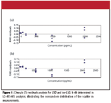
Figure 1

Laboratory management must deal with the extra-analysis issues such as time or money (these are not uncommon) that enter into the balancing equation in the development of a quantitative MS method. From first principles, however, if a published article purports to show a valid quantitative method, the accompanying figures should support that contention. The constraints of space and presentation that accompany the traditional printed publication are relaxed greatly when text, figures, data, and other electronic files are stored and available through a web portal. The community is still in the first stages of setting expectations and standards for such information dissemination, but the transition is inevitable. The accuracy of the information disseminated must be of paramount concern. When data and its interpretation are assessed by impartial colleagues, our community confidence in its integrity is increased. This is "peer review" on a broader scale, with opportunities for increased interactions, more coherent explanations, and effective correction of any errors or misinterpretations.

Before we live in that electronic era in which the dissemination of information is no longer a limiting step, we encounter in our print forums calibration curves used to support a quantitative mass spectrometric analysis. Knowing about uncertainties, errors, and now scedasity, we might be unconvinced of the validity of the curve with only the information presented. Therefore, we conclude this column with a few anonymized examples published recently, view them critically, and suggest a few follow-up questions. The conclusion is not that the data are inaccurate, or the procedures invalid.

Figure 2 plots instrument response (y axis) against sample amount (x axis) for two sample injection methods, with the same amount injected, denoted in the graphs with symbols · or ×. A line (presumably a linear least squares best fit line) is drawn for each of the sample injection methods, thus linking the · and the × points. The conclusion in the article is that results are the same for both injection methods. And yet there are two lines in the figure. The reader cannot ascertain independently that the lines overlap with each other because neither error bars nor confidence limits are given. The reader cannot even know that there are × points at the two lower sample concentrations because they would be obscured by the solid ·. The apparently simple, straight line implies that the data are homoscedastic, but the widening drift between the lines at the upper concentration range suggests that a test for heteroscedasity should be completed.

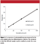
Figure 2

Figure 3 is again a comparison of sample handling/injection methods, with plots of instrument response (y axis) against sample amount (x axis) for two samples. The different symbols represent the three types of injection methods. Note that the range of sample concentration is limited here, spanning perhaps one order of magnitude. The apparent "line" in the figure only connects the data points and is not the result of any analysis. Measurements are clustered at the lower end of the sample concentration range. Neither error bars nor confidence limits are indicated. The data is presented to support the author's choosing one injection method over another, with an assertion that 10–20% more signal will result from that choice.

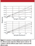
Figure 3

Figure 4 plots instrument response (y axis) against sample amount (x axis) for a gas chromatography (GC)–MS analysis of two targeted chemical compounds. Apparently straight lines connect the data points, and the r² values listed suggest that a regression analysis has been completed. The calibration range starts at 1 μg/mL and extends to a bit over 150 μg/mL. The spacing of the calibration points suggests that the standards were created by serial dilutions (this has an effect through the propagation of errors analysis). Again, neither error bars nor confidence limits are indicated. The spread of data at the lower concentration end is hard to discern in the figure. As in the previous examples, the figure caption is silent on whether the scedasity of the data was established. In this case, the caption is silent as well on the nature of the line (nonweighted or weighted) for which the regression value is listed.

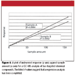
Figure 4

Costs in quantitative MS derive primarily in sample collection, sample preparation, and instrument acquisition and maintenance. Acquisition of repetitive measurements for a given sample adds a relatively small incremental cost. An informed and cogent statistical analysis of the data is without any real cost except the time needed to do so. We have grown to place an incredible confidence in our results because of the sophistication of our instruments. We should not rescind our expectations for a dispassionate assessment of the data that we collect, and a useful and complete presentation of that data.

In addition to the recent texts on quantitative MS, short courses are available that provide an excellent introduction and overview. For example, a two-day course is offered at the annual meeting of the American Society for Mass Spectrometry. The course is based upon a recent text (9), and is offered by C. Basic (Basic Mass Spec, Winnipeg, Manitoba, Canada), R. Bethem (Alta Analytical Laboratory, El Dorado Hills, California), and D.E. Matthews (University of Vermont, Burlington). The course starts with a review of instrumental factors that affect and facilitate quantitation, recognizing that treatment of data is bound to be less than useful when the factors affecting the variances of the data are instrumental in nature. Following a description of statistics to be used, examples are provided that help to assess matrix effects and improve system ruggedness, defined as the suitability of a method for day-to-day operation, in compliance with guidelines and regulations, and with some resistance to disruption. D. Coleman and L. Vanatta write an ongoing series in American Laboratory magazine that deals with statistics in analytical chemistry, and detection limits and calibration issues have been covered in past installments of that series (10,11). Quantitative MS provides vital answers in areas subject to intense scrutiny. Regulation and compliance issues, as well as open assessment and regular review of data, must be integral parts of an analyst's training and expertise.

Kenneth L. Busch once attempted to estimate how many terabytes of MS data are generated on an annual basis, and how much of that total was quantitative data. That estimate, which seemed outrageous just a few years ago, has now been surpassed by reality, and the electronic capability to store, distribute, access, analyze, and discuss that information over the web. It's a brave new world, and KLB grabs his last remaining floppy disk and runs to hide in the Luddite corner. When he comes out, KLB can be reached at wyvernassoc@yahoo.com.

References

(1) M.W. Kiser and J.W. Dolan, LCGC 22(2), 112–117 (2004).

(2) "Guidance for Industry: Bioanalytical Method Validation," United States Food and Drug Administration. Found at http://www.fda.gov/CDER/GUIDANCE/4252fnl.htm.

(3) K.L. Busch, Spectroscopy 23(7), 18–24 (2008).

(4) K.L. Busch, Spectroscopy 22(10), 14–19 (2007).

(5) A.M. Almeida, M.M. Castel-Branco, and A.C. Falcao, J. Chromatogr., B 774, 215–222 (2002).

(6) M. Mulholland and D.B. Hibbert, J. Chromatogr., A 762(1-2), 73–82 (1997).

(7) J.N. Miller, Analyst 116, 3–14 (1991).

(8) Angela Chung, M.S. thesis "Validation of an Ultra Performance Liquid Chromatography Tandem Mass Spectrometry (UPLC/MS/MS) Method for Forensic Toxicological Analysis: Confirmation and Quantitation of Lysergic Acid Diethylamide (LSD) and Its Congeners in Forensic Samples," Toxicology Graduate Program, University of Saskatchewan, Saskatoon, April 2006.

(9) R.K. Boyd, R. Bethem, and C. Basic, Trace Quantitative Analysis by Mass Spectrometry (John Wiley, New York, 2008).

(10) D. Coleman and L. Vanatta, Am. Lab., 28–30 (September 2004).

(11) D. Coleman and L. Vanatta, Am. Lab., 44–46 (February 2008).