Assessing False Noncompliance and False Compliance with Limits Stated for Physicochemical Parameters in Red Wines Using a MIR-PLS Model
Special Issues
When analytical techniques that depend on multivariate calibration models are used to analyze commercial products, the risks of false compliance and noncompliance must be assessed. This study presents an example from the application of a mid-IR partial least squares model to the analysis of seven parameters in red wine.
Several analytical procedures depend on multivariate calibration models, such as partial least squares (PLS) models fitted with near-infrared (NIR) and mid-infrared (MIR) spectroscopy signals. Most of these models are related to products that require the control of maximum (or minimum) legally defined limits so that assessing the risks of false noncompliance and false compliance when establishing the procedure is mandatory. This article shows an application in the field of oenology with red wines from the Spanish qualified denomination of origin (DOC) Rioja, with around 600 samples of wine available, enabling representative training-validation sets. Seven oenological parameters were studied, namely alcoholic degree, total acidity, pH, density, reducing sugar, volatile acidity, and malic acid.
Mid-infrared spectroscopy (MIR) shows great potential for the noninvasive measurement of quality parameters. Consequently, its use is spreading in the world of industry, covering many fields such as agriculture, biotechnology, food and beverages, forensic science, clinical chemistry, pharmaceuticals, and more. The wine sector clearly requires this technology that offers rapid results and low cost.
Fourier transform infrared spectroscopy (FT-IR) is already widespread in wine laboratories and cellars. So much so that the International Organization of Vine and Wine (OIV) has published a guide (1) where the performance of FT-IR partial least squares (PLS) models are explained. This technique can identify the spectral features that can provide information on the factors that affect the quality of alcoholic beverages and, combined with multivariate analysis, increases the chances to obtain quality parameters and their control (2,3). A search in Scopus (01/25/2017) with the keywords “wine” and “MIR” provided 87 publications since 2001, with 33 of them devoted to the determination of parameters in wine. However, no one evaluates the capability of PLS models for fulfilling the legal limits.
Regardless of whether it is a maximum or a minimum limit, when a regulated property is being measured, it is necessary to evaluate the probabilities of false noncompliance and false compliance. For univariate signals, the International Organization for Standardization (ISO) and the International Union of Pure and Applied Chemistry (IUPAC) defined a procedure for determining the detection capability of an analytical method, evaluating the probabilities of false positive and false negative (when an analyte is forbidden). The procedure was generalized for PLS in the literature (4,5) and also adapted to fulfill the official regulation for Zamorano cheese that demands only minimum permitted limits (6).
The MIR spectra combined with PLS regression could be used for the control of the maximum and minimum limits established for the certification of the red wines from Rioja, Spain (7). For this purpose, the new figures of merit CDαand CDβ, analogous to decision limit and detection capability, must be evaluated.
Theory
The PLS regression method is based on latent variables computed as the linear combinations of the predictor variables that are highly correlated with the response variable and, at the same time, explain the variation in the predictor variables (8).
CDα and CDβ
To formalize this section the notation of Commission Decision 2002/657/EC (9) for univariate signals will be used. In particular, permitted limit (PL) is the maximum residue limit, maximum level, or other maximum tolerance for substances established in any normative. When PL = 0, the decision limit (CCα) is the concentration limit at and above which it can be concluded with an error probability of α that a sample is noncompliant when it is. In the case of forbidden substances, for which no permitted limit has been established, the detection capability (CCβ) is the lowest concentration at which a method is able to detect truly contaminated samples with a statistical certainty of 1–β. In the case of substances with an established permitted limit, this means that the detection capability is the concentration at which the method is able to detect permitted limit concentrations with a statistical certainty of 1–β.
The capability of detection in the case of univariate calibration models is well established in the ISO standard 11843 (10) and IUPAC (11). Interestingly, it can be generalized to any type of calibration models (multivariate, multiway, nonlinear, neural-network based, and so on). This generalization is based on the mathematical proof that the capability of detection as is defined by ISO and IUPAC for univariate calibration (signal versus concentration) is invariant for linear transformations of the response (the signal). In particular, the capability of detection is determined by using the concentration predicted with PLS versus true concentration, which is called the accuracy line (y = a + bx) (4,5).
CCα and CCβ, which are defined for PL = 0, are thus generalized for any other value of PL, and named in this paper as CDα and CDβ to distinguish them from the terms already established in other regulations (9–11). Precisely, if it is about a minimum limit, PL = x0 , stated for a given parameter, x, the following hypothesis test is posed:

In equation 1 the null hypothesis H0 is in fact stating that the parameter x is greater than or equal to x0 (that is, the sample is compliant), and thus the alternative hypothesis Ha says that the sample is noncompliant because the parameter x is less than the minimum limit admissible x0.
The decision limit (CDα) of the method is the value of the parameter, below which it can be decided with a probability α that x0 was not reached when it was truly exceeded. Thus, CDα is related to the probability of false noncompliance, α. That is, α is the probability of deciding that the tested sample is noncompliant when it was, the significance level in the hypothesis test of equation 1.
For a given α, the probability β of false compliant decision is the probability of wrongly affirming that the tested sample has a value of the parameter greater than or equal to x0, that is, to conclude that it is compliant, when it was not. The detection capability (CDβ) is the value of the parameter related to this decision.
This is precisely computed as

where Δ(α,β) is the value of noncentrality parameter of a noncentral t-distribution related to the probabilities α and β, ˆσ is the residual standard deviation of the accuracy line, and ˆb its slope, and

depends on the position of the standards in the accuracy line (xi), the number K of replicates and the number of standards I.
When the established limit, PL = x0 is a maximum limit, a similar hypothesis test is used but in this case the alternative hypothesis is Ha: x > x0 (the parameter is greater than x0, so the sample is noncompliant). Thus, the capability of detection CDβ (analogous to CCβ when x0 = 0 in the Commission Decision [9] and to xd in the ISO 11843-1 [10]) is defined by equation 4:

In both cases (minimum or maximum permitted limit, x0 ), the limit of decision CDα (analogous when x0 = 0 to CCα in the Commission Decision and unnamed in the ISO 11843-2) is

where â and ˆb are the intercept and the slope of the accuracy line and yc is the value that satisfies either equation 6 for a minimum permitted limit

or equation 7 for a maximum permitted limit.

Figure 1 shows a schematic representation for an oenological parameter with a minimum limit established, for example the total acidity in Spanish qualified denomination of origin (DOC) Rioja. In this case, the test of equation 1 is applied. As it can be seen, setting the probability α is in practice setting a critical value, yc, (equation 6) that allows the computation of the probability of deciding that a sample does not reach the minimum value when it is false. This statement is related to concentrations CDα (equation 5) and CDβ (equation 2). The concentration CDβ, besides assessing the probability of false noncompliance (α), also assesses false compliance (β). Note that in the value CDα itself, the probability β1 to falsely assert that the wine exceeds the required minimum values is 0.5, while in the concentration corresponding to CDβ this error is reduced to a much smaller amount βn.
Figure 1: Minimum permitted limit Minimum permitted limit (PL). Probability of false compliance, β, as a function of the concentration in an accuracy line (left top corner) and operating characteristic curve (below to the right). The probability of false noncompliance, α, is fixed.
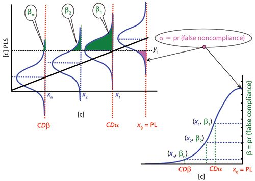
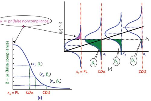
Figure 2 shows the corresponding diagram for a maximum limit. Once the probability α is set, now the critical value yc is determined by equation 7 and CDβ is determined with equation 4. In CDα, the probability β1 of asserting that the wine does not exceed the maximum required limit when it is false is 0.5, whereas in CDβ this probability is largely reduced, βn.
Figure 2: Maximum permitted limit (PL). Probability of false compliance, β, as a function of the concentration in an accuracy line (right top corner) and operating characteristic curve (below to the left side). The probability of false noncompliance, α, is fixed.
In any case, the researcher chooses both risks. The operating curve of the test, the representation of β versus the concentration (for a fixed α) could be used to comparatively examine the performance in the detection capability of several procedures of analysis (or several analyzed parameters).
Experimental
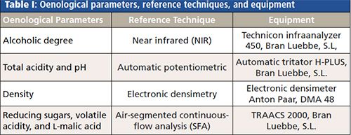
More than 600 samples of red wine are available, all of them analyzed in the official laboratory of the Oenological Station of Haro (La Rioja, Spain) according to official controls with the accredited methods under the norm EN/ISO 17025, number 183/LE407 (Table I). The same samples were scanned, between 1500 and 1000 cm-1 each 5 cm-1 (101 predictor variables), with a Spectrum One FT-IR spectrometer (PerkinElmer) to obtain the MIR spectra. PLS models were computed with PLS Toolbox 5.8.2 2. (11) over Matlab software. CDα and CDβ were estimated using an in-house written program.
Procedure to Build the PLS Models
The procedure consists of the following steps:
1. To build a PLS model for each parameter:
- Preprocess the data matrix X by standard normal variate (SNV). After that, both predictor and response variables are centered.
- Determine the number of latent variables by cross-validation (10 splits data) and compute the root mean squared error in cross-validation (RMSECV).
- Remove those samples with standardized residual (in absolute value) greater than 2.5 or with both Q and Hotelling T2 values larger than their corresponding threshold values at a 99% confidence level.
- Repeat the two previous steps until there are no outliers.
2. To evaluate the predictive capability of the PLS models by using an external set of data with 150 wines. The threshold values of Q and T2 obtained in the calibration step are used to detect outliers by assessing the similarity of the spectra of the evaluation samples with the calibration ones. Moreover, the samples with spectrum similar to those of the training samples but with different values of the calibrated property were also considered outliers. This last assessment is made with the least median of squares regression (LMS) line computed between the PLS predicted values versus the true values of the corresponding parameter. The outliers thus detected were removed and a least squares (LS) regression line was finally fitted. This regression line is the accuracy line, whose characteristics are in the last three columns in Table II for the parameters analyzed.
3. By using the data from the accuracy line, to determine CDα and CDβ with probabilities of both false noncompliance and false compliance fixed at 0.05.
Results and Discussion
The characteristics corresponding to the different PLS models are shown in Table II, in which the slope, intercept, and R2 values corresponding to the accuracy lines obtained with the predicted and true values can be observed too. In all PLS models, the RMSECV values are similar to their corresponding root mean squared error of prediction (RMSEP) values, which indicates stability of the models built. Also, notice that the variance of the oenological parameters (Y) explained by the models is high, ranging from 87.1% to 94.4%, except for the reducing sugar (60.8%).
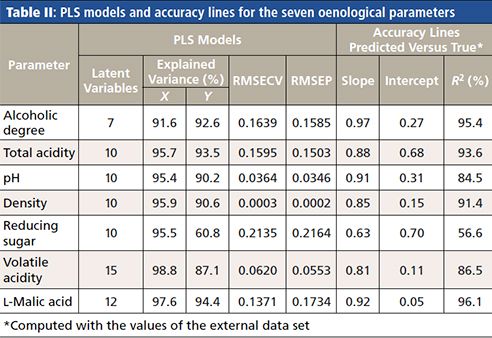
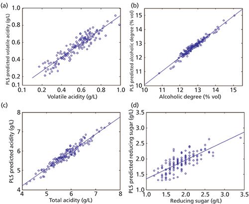
On the other hand, the determination coefficients R2 (explained Y variance) of the accuracy lines with the wines in the external data set are greater than 84.5% (except for reducing sugar). Figure 3 depicts these accuracy lines, only for the models corresponding to the four parameters with compulsory limits. Table III shows the permitted limits and the values obtained for CDα and CDβ for both fitting (the accuracy line is made with the training set) and prediction (wines in the external data set). Also, the number of samples used to compute the values, after deletion of outliers, is shown in Table III.
Figure 3: PLS predicted values versus true values, (a) volatile acidity model, (b) alcohol degree model, (c) total acidity model, and (d) reducing sugar model.
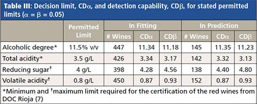
In the case of alcoholic degree the minimum limit established is 11.50% v/v. According to the values in the first row of Table III, the PLS model for this parameter has a CDα in prediction equal to 11.35% v/v. This means that for values less than 11.35% v/v we say that the alcoholic degree of the wine is noncompliant with a 0.05 probability that this assertion is false. But in this case the probability β, to assert that a wine has an alcoholic grade greater than or equal to 11.50% v/v when it is false is 0.50. However, if the PLS model for a wine sample provides a value of 11.23% v/v (equal to CDβ) then β is reduced to 0.05 (see Figure 1).
For a parameter with a maximum limit established-for example, the volatile acidity (last row in Table III)-the values of CDα and CDβ in prediction are equal to 0.87 and 0.93g/L, respectively, when the PL is 0.80g/L. The interpretation is the same for the rest of the parameters with their corresponding values. CDα and CDβ in prediction and fitting are very similar, which means that the values are stable for the future routine use of the PLS models.
Conclusions
All the MIR-PLS models built are highly predictive and stable, for the determination of alcoholic degree, total acidity, pH, density, reducing sugar, volatile acidity, and malic acid in red wines.
This procedure is general, can be applied to products that require the control of maximum (or minimum) legally established limits, and should be taken into account when assessing the risks of false noncompliance and false compliance.
Acknowledgments
The authors thank the financial support provided by the Ministerio de Economía y Competitividad project CTQ 2014-53157-R and FEDER funds.
References
- International Organisation of Vine and Wine, “Resolution OIV-OENO 390-2010,” http://www.oiv.int/en/technical-standards-and-documents/resolutions-oiv/oenology-resolutions (Last access 01/24/2017).
- D.W. Lachenmeier, Food Chem.101, 825–832 (2007).
- C.A. Teixeira dos Santos, R.N.M.J. Páscoa, and J.A. Lopes, TrAC, Trends Anal. Chem. doi:10.1016/j.trac.2016.12.012 (2017).
- M.C. Ortiz, L.A. Sarabia, A. Herrero, M.S. Sánchez, M.B. Sanz, M.E. Rueda, D. Giménez, and M.E. Meléndez, Chemom. Intell. Lab. Syst.69, 21–33 (2003).
- M.C. Ortiz, L.A. Sarabia, and M.S. Sánchez, Anal. Chim. Acta674, 123–142 (2010).
- M.L. Oca, M.C.Ortiz, L.A.Sarabia, A.E.Gredilla, and D. Delgado, Talanta99, 558–565 (2012).
- BOE del 27 octubre de 2004, Ministerio de Agricultura Pesca y Alimentación, 18384 Orden APA/3465/2004.
- H. Martens and T. Naes in Multivariate Calibration (John Wiley and Sons Ltd., Chichester, UK, 1989).
- Commission Decision of 17 August 2002 implementing Council Directive 96/23/EC Concerning the “Performance of Analytical Methods and the Interpretation of the Results” (2002/657/CE), (European Union, Brussels, 2002).
- International Standard ISO 11843-2, “Capability of Detection. Methodology in the Linear Calibration Case” (International Organization for Standardization, Geneva, 2000).
- J. Inczedy, T. Lengyel, A.M. Ure, A. Gelencser, and A. Hulanicki, Compendium of Analytical Nomenclature (IUPAC, Blackwell, Oxford, 1998), chap. 18, pp. 31–40.
- B.M. Wise, N.B. Gallagher, R. Bro, J.M. Shaver, W. Windig, and R.S. Koch, PLS Toolbox 5 (Eigenvector Research Inc., Wenatchee, Washington, 2008).
M.C. Ortiz is with the Faculty of Sciences in the Department of Chemistry at the University of Burgos in Burgos, Spain. L.A. Sarabia and M.S. Sánchez are with the Faculty of Sciences in the Department of Mathematics and Computation at the University of Burgos, Spain. M.E. Meléndez is with the Quality Control Department at the Oenological Station of Haro in Haro, Logroño, Spain. Direct correspondence to: mcortiz@ubu.es
Best of the Week: AI and IoT for Pollution Monitoring, High Speed Laser MS
April 25th 2025Top articles published this week include a preview of our upcoming content series for National Space Day, a news story about air quality monitoring, and an announcement from Metrohm about their new Midwest office.
LIBS Illuminates the Hidden Health Risks of Indoor Welding and Soldering
April 23rd 2025A new dual-spectroscopy approach reveals real-time pollution threats in indoor workspaces. Chinese researchers have pioneered the use of laser-induced breakdown spectroscopy (LIBS) and aerosol mass spectrometry to uncover and monitor harmful heavy metal and dust emissions from soldering and welding in real-time. These complementary tools offer a fast, accurate means to evaluate air quality threats in industrial and indoor environments—where people spend most of their time.