Calibration Transfer, Part IV: Measuring the Agreement Between Instruments Following Calibration Transfer

This is our 100th "Chemometrics in Spectroscopy" column, and when including "Statistics in Spectroscopy," there are now a total of 138 columns. We began in 1986 and have been working since that time to cover in-depth discussions of both basic and difficult subjects. In this newest series, we have been discussing the subject of multivariate calibration transfer (or calibration transfer) and the determination of acceptable error for spectroscopy. We have covered the basic spectroscopy theory of spectroscopic measurement in reflection, discussed the concepts of measuring and understanding instrument differences, and provided an overview of the mathematics used for transferring calibrations and testing transfer efficacy. In this installment, we discuss the statistical methods used for evaluating the agreement between two or more instruments (or methods) for reported analytical results. The emphasis is on acceptable analytical accuracy and confidence levels using two standard approaches: standard uncertainty or relative standard uncertainty, and Bland-Altman "limits of agreement."

As we have discussed in this series (1–3), calibration transfer involves several steps. The basic spectra are initially measured on at least one instrument (that is, the parent, primary, or master instrument) and combined with the corresponding reference chemical information (that is, actual values) for the development of calibration models. These models are maintained on the original instrument over time, are used to make the initial calibration, and are transferred to other instruments (that is, child, secondary, or transfer instruments) to enable analysis using the child instruments with minimal corrections and intervention. We note that the issue of calibration transfer disappears if the instruments are precisely alike. If instruments are the "same" then one sample placed on any of the instruments will predict precisely the "same" result. Because instruments are not alike and also change over time, the use of calibration transfer techniques is often applied to produce the best attempt at model or data transfer. As mentioned in the first installment of this series (1), there are important issues of attempting to match calibrations using optical spectroscopy to the reference values. The spectroscopy measures the volume fractions of the various components of a mixture.

Historically, instrument calibrations have been performed using the existing analytical methods to provide the reference values. These existing methods have often overwhelmingly used weight percents for their results. Until this paradigm changes and analysts start using the correct units for reporting their results we have to live with this situation. We will also have to recognize that the reference values may be some prescribed analysis method, the weight fraction of materials, the volume percent of composition, or sometimes some phenomenological measurement having no known relation to underlying chemical entities, resulting from some arbitrary definition developed within a specific industry or application. Amongst ourselves we have sometimes termed these reference methods "equivalent to throwing the sample at the wall and seeing how long it sticks!" The current assumption is the nonlinearity caused by differences in the spectroscopy and the reported reference values must be compensated for by using calibration practices. This may not be as simple as presupposed, but requires further research.

Multivariate calibration transfer, or simply calibration transfer, is a set of software algorithms, and physical materials (or standards) measured on multiple instruments, used to move calibrations from one instrument to another. All the techniques used to date involve measuring samples on the parent, primary (calibration) and child, secondary (transfer) instruments and then applying a variety of algorithmic approaches for the transfer procedure. The most common approaches involve partial least squares (PLS) calibration models with bias or slope corrections for predicted results, or the application of piecewise direct standardization (PDS) combined with small adjustments in bias or slope of predicted values. Many other approaches have been published and compared, but for many users these are not practicable or have not been adopted and made commercially available for various reasons.

In any specific situation, if the prescribed method for calibration transfer does not produce satisfactory results, the user simply begins to measure more samples on the child (transfer) instrument until the model is basically updated based on the child or transfer instrument characteristics. We have previously described the scenario in which a user has multiple products and constituents and must check each constituent for the efficacy of calibration transfer. This is accomplished by measuring 10–20 product samples for each constituent and comparing the average laboratory reference value to the average predicted value for each constituent, and then adjusting each constituent model with a new bias value, resulting in an extremely tedious and unsatisfying procedure. Such transfer of calibration is also accomplished by recalibration on the child instrument or by blending samples measured on multiple instruments into a single calibration. Although the blending approach improves method robustness (or ruggedness) for predicted results across instruments using the same calibration, it is not applicable for all applications, for analytes having small net signals, or for achieving the optimum accuracy.

How to Tell if Two Instrument Predictions, or Method Results, Are Statistically Alike

The main question when comparing parent to child instrument predictions, a reference laboratory method to an instrument prediction, or results from two completely different reference methods, is how to know if the differences are meaningful or significant and when they are not. There is always some difference expected, since an imperfect world allows for a certain amount of "natural" variation. However when are those differences considered statistically significant differences, or when are the differences too great to be acceptable? There are a number of reference papers and guides to tell us how to compute differences, diagnose their significance, and describe the types of errors involved between methods, instruments, and analytical techniques of many types. The analytical method can be based on spectroscopy and multivariate calibration methods, other instrumental methods, or even gravimetric methods. We have included several of the most noted references in the reference section of this column. One classic reference of importance for comparing methods is by Youden and Steiner (4). This reference describes some of the issues we will discuss in this column as well as details regarding collaborative laboratory tests, ranking of laboratories for accuracy, outlier determination, ruggedness tests for methods, and diagnosing the various types of errors in analytical results.

Let us begin with a set of measurement data as shown in Table I. This is simulation data that is fairly representative of spectroscopy data following multivariate calibration. These data could refer to different methods, such as methods A, B, C, and D; or to different instruments. For our discussion we will designate that the data is from four different instruments A to D for 20 samples. The original data from a calibrated instrument is A1. The results of data transferred to other instruments is represented by B, C, and D. There are duplicate measurements for A as A1 and A2, and for B as B1 and B2, respectively. From these data we will perform an analysis and look for levels of uncertainty and acceptability for the analytical results. Note: C1 and D1 data are used in Figure 2 and will be referred to along with A2 and B2 in the next installment of this column.

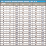
Table I: Data used for illustration, instruments (or methods A, B, C, and D)

Standard Uncertainty and Relative Standard Uncertainty

First, we look at the definitions of uncertainty as described by the United States National Institute of Standards and Technology (NIST), a National Metrological Institute (NMI), which is a nonregulatory agency of the United States Department of Commerce. The lion's share of NIST's purpose is to advance measurement science, measurement standards, and measurement technology. Their charter is to define measurements from first principles that can be verified world-wide and used as standards for making measurements of any kind related to commerce or technology. The NIST definition for uncertainty is quite specific, as explained below (5,6).

Uncertainty Defined

NIST Definitions

The standard uncertaintyu(y) of a measurement result y is the estimated standard deviation of y.

The relative standard uncertaintyu_r(y) of a measurement result y is defined by u_r(y) = u(y)/|y|, where y is not equal to 0.

If the probability distribution characterized by the measurement result y and its standard uncertainty u(y) is approximately normal (Gaussian), and u(y) is a reliable estimate of the standard deviation of y, then the interval y – u(y) to y + u(y) is expected to encompass approximately 68% of the distribution of values that could reasonably be attributed to the value of the quantity Y of which y is an estimate. This implies that it is believed with an approximate level of confidence of 68% that Y is greater than or equal to y – u(y), and is less than or equal to y + u(y), which is commonly written as Y = y ± u(y). The use of a concise notation if, for example, y = 1 234.567 89 U and u(y) = 0.000 11 U, where U is the unit of y, then Y = (1 234.567 89 ± 0.000 11) U. A more concise form of this expression, and one that is commonly used, is Y = 1 234.567 89(11) U, where it is understood that the number in parentheses is the numerical value of the standard uncertainty referred to in the corresponding last digits of the quoted result.

Estimates of Uncertainty

For the data in Table I we simplified our comparison by selecting only A1 and B1 data noting that one might compare multiple analysis for multiple instruments as a more powerful test of the estimated standard deviation of a measurement result for any method or instrument combination. However, the approach shown here is adequate for estimates of uncertainty for typical analysis and calibration transfer applications. We note, using the NIST nomenclature, that

where y is the estimated analytical value for any sample as a function of a series of measurement quantities such as X₁, X₂, . . ., X_N; and where each X_i is an independent observation (or measurement). We also note that when using this nomenclature the A1 and B1 measurements for each sample are denoted as X_i measurements. We note the value (y_i) for each sample measurement is estimated as the sample mean from N independent measurements and is denoted as X_i,k, giving us the relationship as follows.

where N is the total number of X_i (that is, the number of instruments, methods, or models being compared). So our estimated analytical value (y_i) is the mean for a number of measurements of that sample (X(withbar)_i) using the analytical method prescribed. And it follows that the standard uncertainty u(X_i) with reference to the measured values (X_i) is equal to the estimated standard deviation of the mean.

So to apply this to our data illustration from Table I we use A1 and B1 as X₁ and X₂, therefore

where u(y_i) is the estimated standard uncertainty for a series of measurements on multiple samples where the mean value of the measurements for each sample is used for comparison. The equations above are often used for multiple measurements of a single physical constant. For our application using only an A1 and B1 measurement for each sample, we compute the variance for each of the 20 samples and pool the results to give us our estimate of standard uncertainty u(y_i) as

Compiling these results yields the following for the standard uncertainty reported as u(y_i) = 0.226

Relative Standard Uncertainty

This is denoted as u_r (y_i) = u(y_i)/|y_i| and so applying the previously computed results we note that y_iis equal to 14.648 and |y_i| = 14.648 as the mean of all A1 and B1 values. Therefore, the u(y_i) = 0.226 and so the relative standard uncertainty is reported as u_r (y_i)= u(y_i)/|y_i| = 0.226/14.648 = 0.0154.

Confidence Levels Reported:

The confidence levels would be expressed as follows:

For _68%: y _i ± u (y _i) = 14.648 ± 0.226 = 14.42 – 14.87

For _95%: y _i ± 2 . u (y _i) = 14.648 ± 0.452 = 14.20 – 15.10

So the expression of certainty for this example of data would be as y = 14.648 ± 0.226U or y = 14.648(0.226)U.

Thus, for the analyst the final step is deciding if this is a satisfactory result across the two instruments. This concept requires much more discussion, one which we will present in a future column.

Bland-Altman "Limits of Agreement"

For a second look at the data in Table I, we refer to one of the definitive papers used for method comparisons within the highly regulated clinical sciences. We introduce the Bland-Altman method rather than a possibly more familiar calculation because Bland-Altman is the standard for clinical data in an industry with stringent requirements for analytical results. There is an entire series of publications by these statisticians and this method is still taught and used for clinical analysis criteria. One of the possible reasons there are no approved clinical methods using near-infrared (NIR) spectroscopy is that it does not stand up to critical analysis requirements and the NIR groups look at data using unconventional terminology and methods that do not stand up to serious analytical scrutiny. With 27,000 citations in the literature, and having it included in standard university bioengineering curriculum, this would be considered a more standard approach in the wider analytical community. The NIR and chemometric communities would do well to learn from these older and thoroughly tested methodologies and referenced papers.

The paper we cite is entitled "Statistical Methods for Assessing Agreement Between Two Methods of Clinical Measurement," and was written by J. Martin Bland and Douglas G. Altman (7). This paper describes the errors often made when comparing methods. The authors summarize the contents of this paper as follows, "In clinical measurement comparison of a new measurement technique with an established one is often needed to see whether they agree sufficiently for the new to replace the old. Such investigations are often analyzed inappropriately, notably by using correlation coefficients. The use of correlation is misleading. An alternative approach, based on graphical techniques and simple calculations, is described." So, what can be learned by using the techniques described in this paper to compare results from analytical methods? When methods are compared following calibration, one attempts to assess the degree of agreement between them. Bland and Altman discount completely the use of correlation as a useful parameter to assess analytical agreement. Their arguments are given in this discussion.

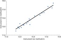
Figure 1: Instrument or method A1 (x-axis) as compared to instrument or method B1 (y-axis), and with data points compared to perfect line of equality.

For this method comparison, two single measurements are taken for each sample on each instrument as A1 and A2. The first measurement is used for comparison and the second for a repeatability study (which we will cover in a later installment). For this method of comparison a line of equality plot is made to compare two methods or two instruments. The various x, y data points are plotted against a perfect straight line of equality. The authors make the point that correlation (r) measures the strength of the relationship between two variables, but it does not measure the agreement between them (Figure 1). Perfect agreement is indicated by the data points lying directly on the line of equality. A perfect correlation is indicated if all the points lie along any straight line. The authors emphasize that: correlation indicates the strength of a relationship between variables — not that the analytical results agree; a change in scale does not affect correlation, but drastically affects agreement; correlation depends on the range of the true quantity (analyte) in the sample; tests of significance are mostly irrelevant between two similar analytical methods; and data in poor agreement analytically can be highly correlated (Figure 2). Figure 2 shows three analytical sets with perfect correlation but poor agreement.

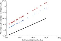
Figure 2: Instrument or method A1 (x-axis) as compared to instruments (or methods) C or D (y-axis), showing line of equality for perfect agreement as well as other perfect correlations that are not in analytical agreement. This indicates correlation as an imperfect representation of agreement between methods.

A Bland-Altman plot shown in Figure 3, which will be extremely familiar to clinical analysts, demonstrates a good visual comparison technique to evaluate the agreement between two methods or instruments. The x-axis (abscissa) for each sample is represented by the average value for each sample obtained from the comparison results (using two methods or two instruments). The y-axis (ordinate) for each sample is represented by the difference between one method and the second method (or instruments A and B in our example) for each sample. Such a plot uses the mean and plus or minus two standard deviations as the upper and lower comparison thresholds.

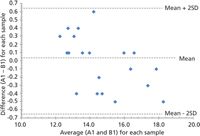
Figure 3: The Bland-Altman plot indicating the difference plotted against the mean for each sample for instrument (or methods) A1 and B1. (Note: For random, normally distributed data we would expect one sample out of 20 to be outside the ±2 SD range.)

To assess if the data are in close enough agreement for our analytical purposes between A1 and B1 we compute the bias or mean difference (d(withbar)), the standard deviation of the differences (s or SD), and the expected "limits of agreement." These are expressed as d(withbar) ± 2s for a 95% confidence level.

The mean difference is computed as the average of all the differences between the comparative instruments, for each sample as

The standard deviation for this comparison for the set of samples is computed as

And so for our data A1 and A2 in Table I we find the following results: Bias is d(withbar) = -0.226; standard deviation for all samples is s = -0.015; 95% confidence level is d(withbar) + 2s = 0.438 and d(withbar) – 2s = -0.468.

If this number is considered too large for a 95% confidence of the result agreement then these methods are not considered equivalent. On the other hand if these limits of agreement are acceptable for the application where they are used, then this is acceptable. In a clinical situation, a physician determines the level of accuracy or agreement required for critical intervention decision making; this would be analogous to a process control supervisor or analytical scientist assessing the acceptable level of agreement between comparative methods to use the alternate method or instrument as a substitute.

Conclusion

These two similar, classic, and well-accepted methods have been applied to analytical results in commerce and clinical analysis. Included below are references for the reader's further study of this subject of comparing two or more analytical methods or instruments. Other references discussing the details of comparing analytical methods are also provided (8–16).

References

(1) H. Mark and J. Workman, Spectroscopy28 (2), 24–37 (2013).

(2) H. Mark and J. Workman, Spectroscopy28 (5), 12–25 (2013).

(3) H. Mark and J. Workman, Spectroscopy28 (6), 28–35 (2013).

(4) W. Youden and E.H. Steiner, Statistical Manual of the AOAC, (Association of Official Analytical Chemists, Arlington, Virginia, 1984).

(5) http://physics.nist.gov/cgi-bin/cuu/Info/Constants/definitions.html.

(6) B.N. Taylor and C.E. Kuyatt, "Guidelines for Evaluating and Expressing the Uncertainty of NIST Measurement Results" (NIST Technical Note 1297, September 1994 Edition).

(7) J.M. Bland and D.G. Altman, Lancet1, 307–10 (1986).

(8) W. Horwitz, Anal. Chem.54 (1), 67A–76A (1982).

(9) P. Hall and B. Selinger, Anal. Chem. 61, 1465–1466 (1989).

(10) D. Rocke and S. Lorenzato, Technometrics37(2), 176–184 (1995).

(11) J.C. Miller and J.N. Miller, Statistics for Analytical Chemistry, Second Edition (Ellis Horwood, Upper Saddle River, New Jersey, 1992), pp. 63–64.

(12) W.J. Dixon and F.J. Massey, Jr., Introduction to Statistical Analysis, Fourth Edition), W.J. Dixon, Ed. (McGraw-Hill, New York, 1983), pp. 377, 548.

(13) D.B. Rohrabacher, Anal. Chem.63, 139 (1991).

(14) H. Mark and J. Workman, Chemometrics in Spectroscopy (Elsevier, Academic Press, 2007), Chapters 34–39, 71–73.

(15) ASTM E1655 - 05 (2012) Standard Practices for Infrared Multivariate Quantitative Analysis (2012).

(16) H. Mark and J. Workman, Statistics in Spectroscopy, 2nd Edition (Elsevier, Academic Press, 2003), Chapter 7, pp. 59–69.

Jerome Workman, Jr. serves on the Editorial Advisory Board of Spectroscopy and is the Executive Vice President of Engineering at Unity Scientific, LLC, (Brookfield, Connecticut). He is also an adjunct professor at U.S. National University (La Jolla, California), and Liberty University (Lynchburg, Virginia). His e-mail address is JWorkman04@gsb.columbia.edu

Jerome Workman

Howard Mark serves on the Editorial Advisory Board of Spectroscopy and runs a consulting service, Mark Electronics (Suffern, New York). He can be reached via e-mail: hlmark@nearinfrared.com

Howard Mark