Choosing the Best Regression Model
Spectroscopy
When using any regression technique, either linear or nonlinear, there is a rational process that allows the researcher to select the best model.
When using any regression technique, either linear or nonlinear, there is a rational process that allows the researcher to select the best model. One question often arises: Which regression method (or model) is better or best when compared to others? This column discusses a mathematical and rational process that is useful for selecting the best predictive model when using regression methods for spectroscopic quantitative analysis.
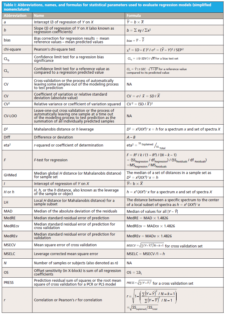
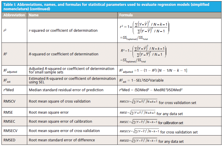
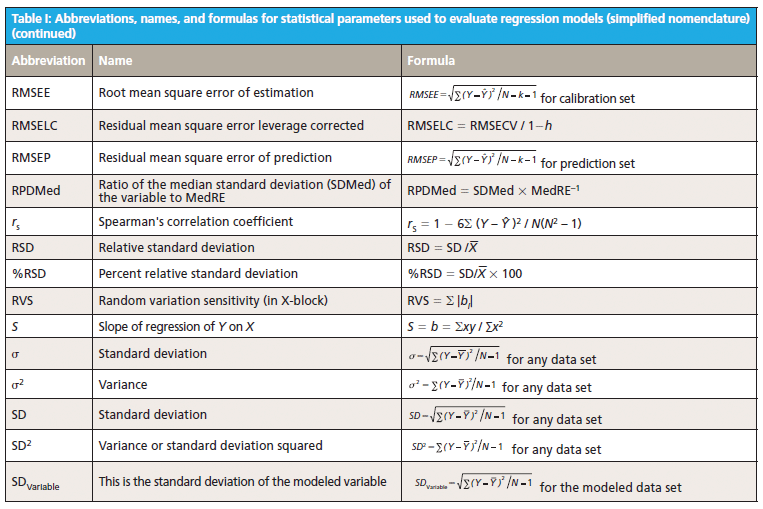
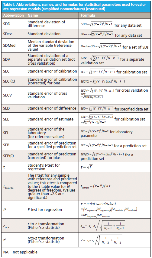
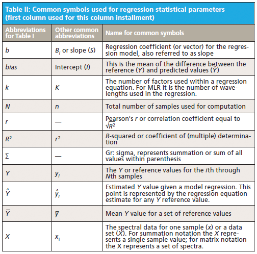
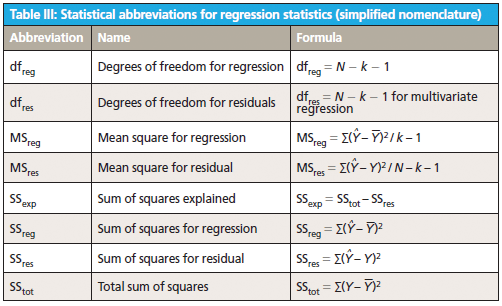
This column does not address the mathematics for optimizing regression modeling; it does however address the selection of an optimized model after it has been developed. Guidelines for the experimental design of the calibration and validation processes are included. Standard techniques for comparing regression results include familiar methods: bias, slope, standard error of calibration, standard error of prediction, standard error of cross validation, standard error of validation, correlation, coefficient of determination, r-to-z transform (that is, Fisher's z-transform), prediction errors (of various types), and the coefficient of variation (1,2). Table I outlines the various standard methods using simplified nomenclature with essential symbols and abbreviations further described in Tables II and III.
Less used statistics for spectroscopy include the comparison of slopes using analysis of covariance (ANCOVA) (3), the empirical distribution function (EDF) (4), the Anderson-Darling statistic (5), the Durbin-Watson statistic (6), the receiver operating characteristic (ROC), and ROC curves that are useful for comparing analysis quality (7). Simple linear and multiple linear regression allow the familiar parametric statistics and hypothesis tests including the F-statistic and Student's t-statistic, along with the probability levels, to compare the basic goodness of fit for the regression for X versus Y data (8–10). In addition, one may find references relating to the sum and average absolute differences from zero of the regression coefficients themselves as having distinct interpretation and significance (11).
Regardless of the complexity of regression method used, the degree of polynomial, or whether linear or nonlinear methods are used to fit the calibration data, the basic feature required for the best model is sensitivity of the model to predict Ŷ from spectral (X) inputs accurately and precisely over time. The main quantity used for evaluating this is to determine the difference between predicted values for a model (designated as Y) and the reference or actual values used to create the model (designated as Ŷ) under rigorous conditions. More-detailed research literature has described many statistical parameters useful for regression validation or testing (11,12).
Goodness of fit is defined as how well a regression model fits the set of observations as reference or expected values (Ŷ) versus the regression predicted values (Ŷ). The difference between expected and observed values is the main criterion for selecting model fitness, assuming the calibration and prediction experiments are properly derived. There are many residual (Y – Ŷ) based parameters used to measure the fitness of any regression model (Tables I–III); however, true residual tests indicative of model fitness must include aspects of robustness or rigor to properly test the model or regression capacity for accurate predictions for all types of samples. In other words, the key criteria for the best model are how well a regression model predicts samples that were not used to build or compute the original model, and how well the prediction results hold when samples are predicted over time and under changing conditions. For goodness of fit determination for any regression, statistics such as the lack of fit sum of squares as root mean square error of cross validation (equation 1) and the coefficient of determination (equation 2) are the main criteria for comparing model fitness. More will be said about these parameters later, noting that the correlation is not necessarily related to prediction error.

The calculated fitting parameters and experimental design specifics for the calibration and prediction data are paramount for determining the best regression model for any specific application. It is the best mathematical model that when applied to spectra obtained from a sample of unknown concentration will compute a reliable, accurate, and reproducible value of composition, as weight or moles per unit volume, for the components of interest. The ideal mathematical model will be insensitive to normal instrument variation, temperature effects, background interferences, ambient humidity, and vibration; at the same time it will be most sensitive to changes in the concentration of the components of interest. Proper experimental design of the calibration and validation processes yields superior results in terms of measurement precision, accuracy, sensitivity, and selectivity for analyte predictions. Under typical conditions, the rigor of the experimental design determines the effectiveness of calibration modeling and validation testing.
Multivariate modeling is required when the spectra of analyte components within a sample mixture are overlapped in spectral space. For multivariate regression models to be optimized, they must include regression coefficient amplitude weightings (for principal components regression [PCR] and partial least squares [PLS]) or wavelength selection (for multiple linear regression [MLR]) where the molar absorptivity values for each analyte present in the sample matrix are the most different. In MLR, the analyst assumes that adding new or different factors or wavelengths will provide a calibration equation compensating for random instrument noise and drift, chemical interferences, nonlinearity in detectors and electronics, background scattering, and other perturbations normally encountered when measuring samples and recording spectra (13–20).
Optimizing the Experimental Design for Calibration
A basic calibration experiment must be well constructed for success. The optimum calibration set includes specific variables such as instruments, sample holder, sample types, particle sizes, moisture content, lot or crop year, manufacturing plant or geographic differences, and operators for preparing and presenting samples. Other variables would include chemical interferents, pathlength variation, flow differences (flow cells), ambient temperature and humidity, environmental vibration, optical sources, sampling device, and the like. For natural products, phenotype and geographical region as well as crop year must be included. A recommended recipe for calibration and validation experiments would be as follows:
1. Collect enough samples to cover the entire set of experimental values as listed above for all constituents of interest (21–23).
2. Carefully measure spectra of selected samples (replicates are best).
3. Use a sample selection algorithm to reduce the sample set to a manageable size while eliminating redundant samples and including unique samples (24,25).
4. Perform the conventional reference chemical analysis on selected samples. The reference methods must be as accurate as possible. The chemical values used must be the mean results for a minimum of blind duplicate analyses using an official chemical analysis procedure. The laboratory values should be audited with known precision and accuracy.
5. There should be little or no intercorrelation or covariance between the major predicted constituents unless the relationship always exists within this type of material (26).
6. The calibration model is created and tested using cross-validation or separate validation such as standard error of cross validation (SECV) and predictive residual sum of squares (PRESS) (see Table I). These values are to be the smallest for a series of rigorous cross-validation tests.
7. Multiple validation sample sets are held aside for prediction testing and are set up to contain all potential variables. These include, but are not limited to, variations in particle size, sample preparation, instrument, operator, and sample types (22,23).
8. Overall quality of the calibration is tested for the validation sets using the statistical methods found within Table I, these include standard error of calibration (SEC), root mean square error of cross validation (RMSECV), SECV, PRESS, standard deviation (SDV), bias, confidence limit test for a regression bias significance (CLb), confidence limit test for a reference value as compared to a regression predicted value (CLr), offset sensitivity (OS), and random variation sensitivity (RVS) and other residual based tests (as preferred). Note that correlation and the coefficient of determination are not good tests for comparison of regression models for selection of the optimum model as correlation is dependent on the constituent range and is not a predictor of error. High correlation may exist coincidently with high error (27).
9. The regression vector or wavelengths used in the calibration model should match the vibrational absorbance frequencies known to correspond to the constituents of interest (28,29).
10. A validation sample set should be used to determine approximate standard error value and this is tested using the confidence limit statistic as equation 3. Individual reference sample values should lie within the range of the upper and lower confidence limits above and below the predicted value (12).

The t value is selected for the 95% confidence limit for N – k – 1 degrees of freedom. This would be 1.96 for a typical calibration set of greater than from 125 to 130 samples. Thus, an appropriate calibration would have 95% or more of all reference samples falling within this confidence limit. The larger the percentage of reference samples falling within this confidence limit, for each sample and each model, the better is the regression model.
11. Monitor the selected calibrations using a periodic difference test (or bias test) as compared to a set of reference test validation samples. The bias test set is analyzed carefully by the reference method and represents the current crop conditions or manufacturing process conditions. The bias confidence limit (Y with bar - Ŷ with bar) is as shown in equation 4.

For the bias to not be significant it must be within the confidence limits for the number of samples used to test the bias. Note that t = 2.23 for N = 10, 2.13 for N = 15, 2.09 for N = 20, and 2.06 for N = 25 (at the 95% confidence level). N is the number of samples used to test the bias.
Validating the Regression Model
Validation of each multivariate regression model is tested by applying the model to a separate set (or sets) of validation samples. The differences between the predicted results and the reference results are a partial proof of optimized models (given a complete and thorough calibration development process). Validation of a model requires certain complex characteristics for a validation set. The validation set must have the following characteristics.
- All chemical interferents expected in routine analysis must be included within the sets.
- The range of constituents must closely approximate the samples that will be measured routinely.
- There should be a uniform distribution of the chemical parameters or constituents to be measured.
- There should be a comprehensively large validation set, possibly as many as 100 or more test samples. As a minimum, the number of validation samples should exceed four-times the number of factors (or wavelengths in the case of MLR) used to develop the model.
- The validation set must consist only of samples that test an interpolation of the model, since predicting samples representing extrapolation of the model is not recommended. In other words, the validation samples should be within the calibration space and not considered to contain outlier samples.
- The validation set should span approximately 95% of the concentration range for any constituent.
- Compute at least the following parameters for each calibration to be compared: SEC, RMSECV (SECV), PRESS, SDV, bias, CLb, CLr, OS, and RVS.
Summary
In comparing appropriate calibration and validation experiments a spreadsheet showing the computed values for SEC, RMSECV (SECV), PRESS, SDV, bias, CLb, CLr, OS, and RVS for each equation will allow the user to quickly assess the most superior or best model. The best model will have the smallest values for each parameter. There are other useful statistics listed within the literature as shown in the references, however for calibration using spectroscopy, these validation statistics will yield the greatest information in an efficient manner for selection of the best calibration for routine use. Remember that the calibration and validation sets must be carefully composed for confidence in routine analysis. One may rank the equations from best to worst based on the lowest to highest values for this set of parameters.
References
(1) H. Zar, Biostatistical Analysis, 5th Ed. (Pearson, New Jersey, 2009).
(2) D.F. Polit, Statistics and Data Analysis for Nursing Research, 2nd Ed. (Pearson, New Jersey, 2010).
(3) D. Rogosa, Psychological Bulletin 88(2), 307–321 (1980).
(4) M.A. Stephens, J. Am. Stat. Assoc. 69(347), 730–737 (1974).
(5) F. Laio, Water Resour. Res. 40(9), W09308, 1–10, (2004).
(6) R.J. Hill and H. D. Flack, J. Appl. Crystallogr. 20(5), 356–361 (1987).
(7) E.A. Nadaraya, Theory Probab. Its Appl. 9(1), 141–142 (1964).
(8) H.A. Martens and T. Naes, Multivariate Calibration, 1st Ed. (John Wiley and Sons, New York, New York, 1993).
(9) H. Mark and J. Workman Jr., Statistics in spectroscopy, 2nd Ed. (Elsevier, Academic Press, 2003).
(10) H. Mark and J. Workman Jr., Chemometrics in Spectroscopy, 1st Ed. (Elsevier, Academic Press, 2010).
(11) J. Workman, in Handbook of Near-Infrared Analysis, 3rd Ed., D. Burns and E Ciurczak, Eds. (CRC Press, Taylor and Francis, 2008), pp. 137–150.
(12) ASTM E1655 - 05(2012), Standard Practices for Infrared Multivariate Quantitative Analysis, ASTM International, 100 Barr Harbor Drive, PO Box C700, West Conshohocken, PA, 19428-2959 USA, 2012.
(13) P.M. Fredericks, P.R. Osborn, and P.R. Swinkels, Anal. Chem. 57(9). 1947–1950 (1985).
(14) W.J. Kennedy and J.E. Gentle, Statistical Computing (Marcel Dekker, New York, New York, 1980).
(15) S. Wold, H. Martens, and H. Wold, in Matrix Pencils (Springer Berlin Heidelberg, 1983), pp. 286–293.
(16) H.-W. Tan and S.D. Brown, J. Chemom. 16(5), 228–240 (2002).
(17) W. Lindberg, J. Persson, and S. Wold, Anal. Chem. 55(4), 643–648 (1983).
(18) P. Geladi and B.R. Kowalski, Anal. Chim. Acta 185, 1–17 (1986).
(19) D.M. Haaland and E.V. Thomas, Anal. Chem. 60(11), 1193–1202 (1988).
(20) B. Godin, R. Agneessens, J. Delcarte, and P. Dardenne, J. Near Infrared Spectrosc. 23(1), 1–14 (2015).
(21) D. Abookasis and J. Workman, J. Biomed. Opt. 16(2), 027001–027001 (2011).
(22) T. Næs and T. Isaksson, Appl. Spectrosc. 43(2), 328–335 (1989).
(23) T. Isaksson and T. Næs, Appl. Spectrosc. 44(7), 1152–1158 (1990).
(24) D.E. Honigs, G.M. Hieftje, H L. Mark, and T. B. Hirschfeld, Anal. Chem. 57(12), 2299–2303 (1985).
(25) J.S. Shenk and M.O. Westerhaus, Crop Sci. 31(2), 469–474 (1991).
(26) P.M. Bentler and D.G. Bonett, Psychological Bulletin 88(3), 588–606 (1980).
(27) J.M. Bland and D.G. Altman, J.-Lancet 327(8476), 307–310 (1986).
(28) J. Workman and L.Weyer, Practical Guide and Spectral Atlas for Interpretive Near-Infrared Spectroscopy, 2nd Ed. (CRC Press, Taylor and Francis, Florida, 2012).
(29) F. Westad, A. Schmidt, and M. Kermit, J. Near Infrared Spectrosc. 16(3), 265–273 (2008).
Jerome Workman, Jr. serves on the Editorial Advisory Board of Spectroscopy and is the Executive Vice President of Engineering at Unity Scientific, LLC, in Brookfield, Connecticut. He is also an adjunct professor at U.S. National University in La Jolla, California, and Liberty University in Lynchburg, Virginia. His e-mail address is JWorkman04@gsb.columbia.edu

Jerome Workman, Jr.
Howard Mark serves on the Editorial Advisory Board of Spectroscopy and runs a consulting service, Mark Electronics, in Suffern, New York. He can be reached via e-mail: hlmark@nearinfrared.com

Howard Mark
