Classical Least Squares (CLS), Part 3: Expanding the Analysis to Include Concentration Information on Principal Component Regression (PCR) and Partial Least Squares (PLS) Algorithms
We explore how different algorithms and different numbers of factors affect the results.
From the spectra alone, we have been able to deduce some interesting things about the behavior of data. We can now extend our data analysis to apply algorithms that include the constituent information as well. This article examines the behavior of data when subjected to the popular principal component regression (PCR) and partial least square (PLS) algorithms. PCR is essentially the same as principal component analysis (PCA), but it takes the results a little further by relating them to known information about the composition or other characteristics of the material being studied.
This is our first exploration into evaluating the effect of using an advanced calibration algorithm on calibration performance. We also look at the effects of different algorithms, different numbers of factors for both principal component regression (PCR) and partial least squares (PLS) algorithms, and different ways to look at the results. Although we do not eschew use of the simple numerical measures commonly used to evaluate calibration performance, we consider the way the common diagnostic statistics change under the different conditions to be of much greater importance. Therefore, the bulk of our article here consists of graphical displays that provide much more information that the raw numbers alone.
Figures 1, 2, 3, and 4 show the results of applying the PCR and PLS calibration algorithms to the same spectral data. For each algorithm, volume fractions and weight fractions served as the constituent values. The results are summarized as the residual variance. Table I presents the organization of these four figures.

As we reported in our previous column on this topic (1), the use of five chemical components to construct the sample set means that theoretically there should be only four degrees of freedom in the data set. Despite that, we discovered that some of the analytes required the use of up to six PCR or PLS factors. However, artifacts revealed in the results already presented (such as the patterns of residuals seen in the data plots) indicate that there is more to the story. To ensure that we did not miss any important effects, we continued the calculations for both PCR and PLS analysis to include all numbers of factors up to ten factors, for each calibration, and we report all of those results.
Effect on PCR Analysis
Figure 1 shows the effect on the residual variance of volume fractions. The residual variance is the basic measure of the error of the constituent value, from which statistics such as the standard error of estimate (SEE) and standard error of calibration (SEC) are calculated. Principal component analysis (PCA) is used to generate the model and the constituent is presented as volume fraction. Figure 1 shows the residual variance for each ingredient at the different stages, where they have various numbers of principal components included in the calibration.
Figure 1: Residual variance from PCR calibrations for varying numbers of principal components included in the calibration calculations and using volume fractions as the constituent concentrations. Important features of the behavior of the data are marked. See text for full explanation.
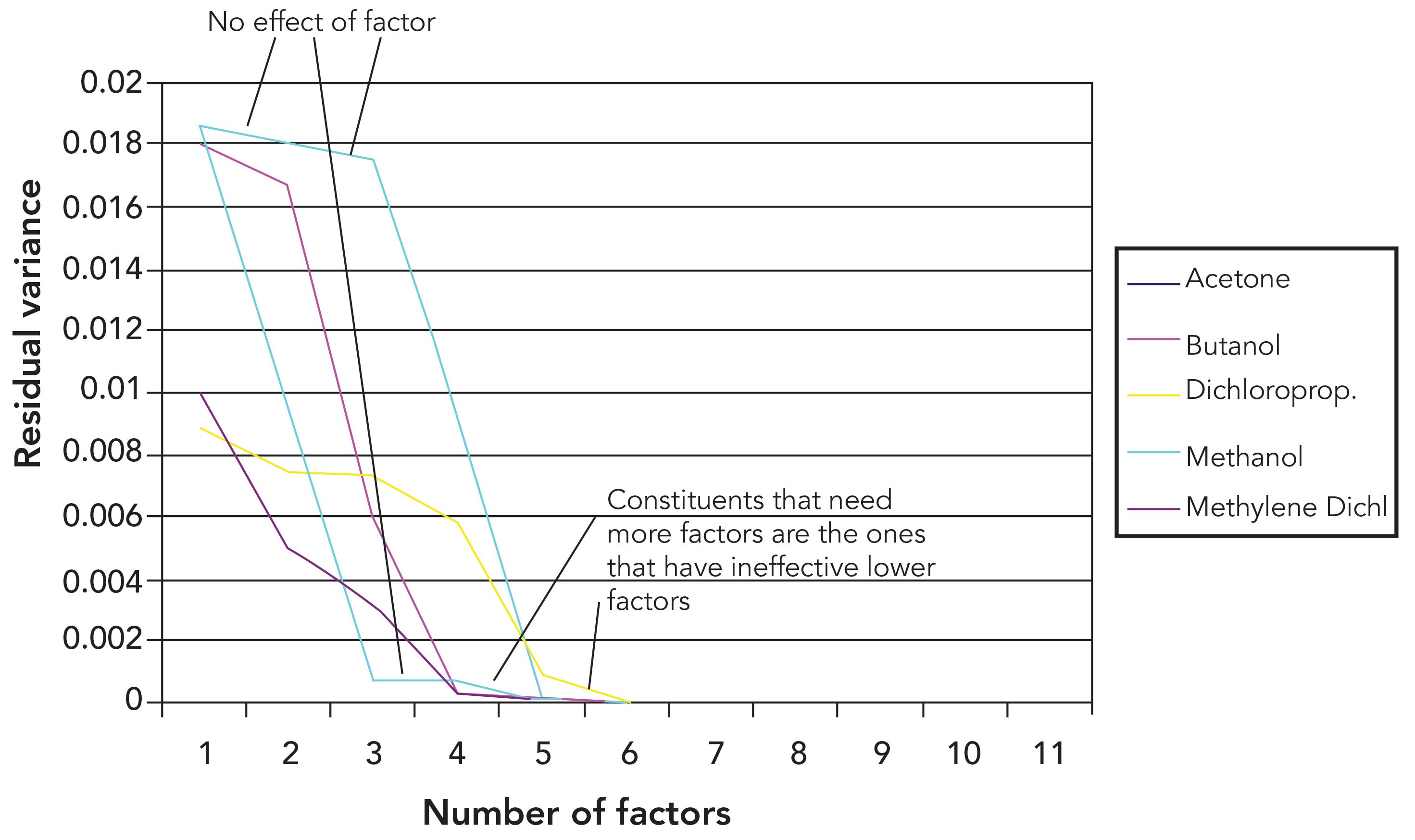
We note in Figure 1 that changes in calibration performance depend on the number of principal components used. Some of the ingredients (such as methanol and methylene dichloride) show large improvements in the calibration performance for early principal components (PCs), whereas for others (such as butanol and dichloropropane) no appreciable improvement in calibration performance was noted until three or more PCs have been included in the calibration model. This observation is consistent with the behavior we observed in the previous installment, where the variance of the spectra also required more than the theoretical number of PCs (four). We also note in Figure 1 that for these latter two ingredients, at least one early PC makes no contribution to improvement of the performance of the calibration model, as marked in the figure.
The calibration performance of these various ingredients is complicated to describe. Acetone and dichloropropane are two ingredients that required more than four PCs to produce a calibration where the residual error approached the noise level. Those two ingredients are also the ones for which one or more early PCs make very little contribution to their calibration performance. Dichloropropane showed some improvement when the second PC was included in the calibration model, but the third PC did little to improve it further. For methylene dichloride, neither of the first two PCs appreciably improved the calibration performance. For both of those ingredients it required more than four PCs to improve the performance values to be comparable to the other ingredients. It thus appears that each ingredient individually requires four PCs to achieve an optimum calibration. However, depending on the ingredient, these four PCs are not necessarily the first four PCs that are computed from the spectral variations. This finding explains that the previous observation (1) required six PCs to account for the total spectral variability in the data. It is here that we see the underlying cause of that behavior: Some of the PCs do not explain the variance of some of the mixture constituents. Therefore, it requires more PCs than expected to account for all the variance caused by all the ingredients, even if only a few of the ingredients require the higher principal components.
Both butanol and methylene dichloride had virtually all of their respective variances accounted for by the point where four PCs have been included in the calibration model. As we see, both of these ingredients are indistinguishably close to the x‑axis by the point where four PCs are included in the model. Moreover, while dichloropropane required the full six PCs to reach zero residual variance, acetone only required five despite the fact that the first two PCs made little contribution to the calibration performance for this ingredient; all the “heavy lifting” for this constituent was done by PCs 4 and 5. For butanol, the major contribution to calibration performance is attributed to PCs 3 and 4.
Now let’s compare the results from calibrating for weight fractions to what happens when the constituent concentrations are expressed as volume fractions. Figure 2 presents the application of the PCR algorithm on the dataset we have been exploring, using the weight fraction for the “concentration.” This is exactly analogous to our previous discussion except using weight fractions instead of volume fractions.
Figure 2: Residual variance from PCR calibrations for weight percent. This figure shows varying numbers of principal components included in the calibration calculations and uses weight fractions as the constituent concentrations. Analytes that require more than four PCs are the ones where the lower PCs had no effect. In all cases, four PCs explain the variance in the spectra, but not necessarily the first four PCs.

Comparing the effects on performance in Figure 1 with the corresponding ones in Figure 2, we see that the same effects are operative. In Figure 1, however, the way they affect the performance‑versus‑number of PCs agreement in a clearer way than in Figure 2. On the other hand, there is the same tendency for only two of the PCs to account for most of the reduction in error, for acetone, methanol and butanol, as there was when the analyte concentration was expressed as volume fraction in Figure 1.
We noted above that for acetone and butanol the value of the residual variance became indistinguishable from the x‑axis when the first four PCs are included in the model. When weight fractions are used for the constituent concentrations, however, there is still some variance not accounted for at that point, as evidenced by the fact that for both constituents, there is a noticeable space between the graph point corresponding to four PCs and the x‑axis, when the units of the constituent are weight fractions.
This is a fine point, but it raises an important question: Why is the residual variance for four PCs smaller when volume fractions are used? We attribute that behavior to the fact that the first four PCs are in fact enough to account for the real spectral variability of the data when volume fractions are used, and this is consistent with our previous findings. When weight fractions are used to describe constituent concentrations, however, there is additional variance due to the nonlinear relationship between this component “concentration” value and the spectral data. This excess variance is not present when volume fractions are used; therefore, there is no excess variance to show up in the volume–fraction plot.
The same PCs are computed in both cases (because the computation of PCs do not involve the constituent values), and because PCs are orthogonal, those that improve the calibration performance will make the same contribution to that improvement regardless of the presence or absence of other PCs. Thus, equivalent calibration performance for any given ingredient should be obtainable by including only those PCs in the calibration model that contribute to the improvement of the performance for that ingredient, answering the question posed above (“why is the residual variance for four PCs smaller when volume fractions are used?”). The answer to that question is based on the same considerations we concluded previously: The excess PCs are attempting to compensate for the nonlinear behavior of the relationship between the weight fraction and the spectroscopic measurement. Thus we see that it is not necessary, and indeed it is to be likely counterproductive, to include excess numbers of PCs in a calibration model (conventionally called “overfitting”) solely because the software being used requires that all PCs from the first to the nth be included in the model. If nothing else, it will add unnecessary noise to the results of the computation.
Effect on PLS Analysis
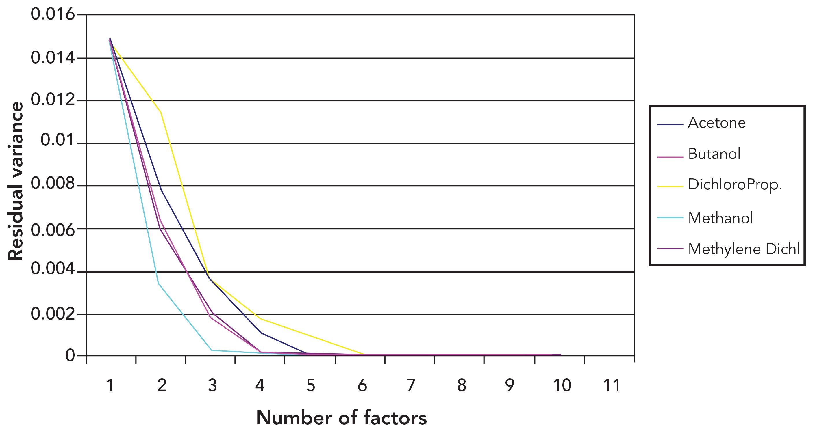
Figures 3 and 4 present graphs corresponding to Figures 1 and 2 but show the results of performing PLS analysis on the data instead of PCR analysis. Not surprisingly, the graphs are very different from the ones in Figures 1 and 2. This results from the nature of the two algorithms and the differences between them. The extraction of the spectral variance by PCR is performed independently of the constituent values, and each PCR loading indicates only the actual changes that result from the spectra of the constituents and their respective concentrations. As we noted above, the same PCR loading is therefore calculated regardless of the constituent under consideration for the calibration. In the case of PLS, however, the calculation of each loading includes a contribution from the constituent for which the calibration is being performed, and each loading differs from the corresponding loadings for the other constituents. The result is that each PLS loading is optimized for the constituent it was generated to calibrate for, and therefore includes the maximum amount of variance from that constituent. It is nearly impossible, therefore, for any PLS loading to not include some of the remaining variance in either the constituent or spectral values; therefore, there cannot be any PLS loadings which do not remove variance from the data as, for example, the second and third PC did for acetone in Figure 1, or the third PC did for dichloropropane, in Figure 1.
The mathematical properties of the PLS analysis thus overwhelms the inherent properties of the spectral data itself while some small vestiges remain. Figure 3 notes the shape and rate of descent of the plotted values of the residual variance of acetone, and compares that with the corresponding plotted values of dichloropropane in Figure 4. In both cases, the specified values of residual variance are the largest in their respective plots; furthermore, the shapes of these two plots are very similar. Similar effects can also be seen for all the other constituents as well.
Figure 3: Residual variance from PLS calibrations for varying numbers of principal components included in the calibration calculations, and using volume fractions for the constituent concentrations.
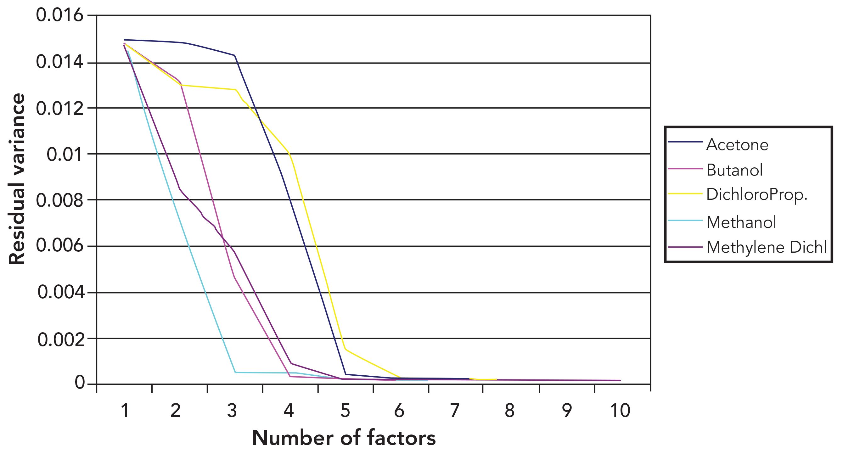
Figure 4: Residual variance from PLS calibrations, for varying numbers of principal components included in the calibration calculations, and using weight fractions for the constituent concentrations.
Although we cannot include all the graphs we created in this column, we would be remiss if we did not include at least a minimum number of examples of the utility of examining residual plots. Figure 5 presents two residual plots for dichloropropane. These plots are both results obtained from performing PCR analysis of the data, and plotting weight fractions and volume fractions, respectively, against the PCR predicted values. The curvature of the weight fraction plot is observable while the corresponding plots using volume fractions can be seen to be free from any noticeable nonlinearity.
Figure 5: PCR predictions for dichloropropane using five principal components. (a) Residuals for weight fractions versus predicted values and (b) residuals for volume fractions versus predicted values.
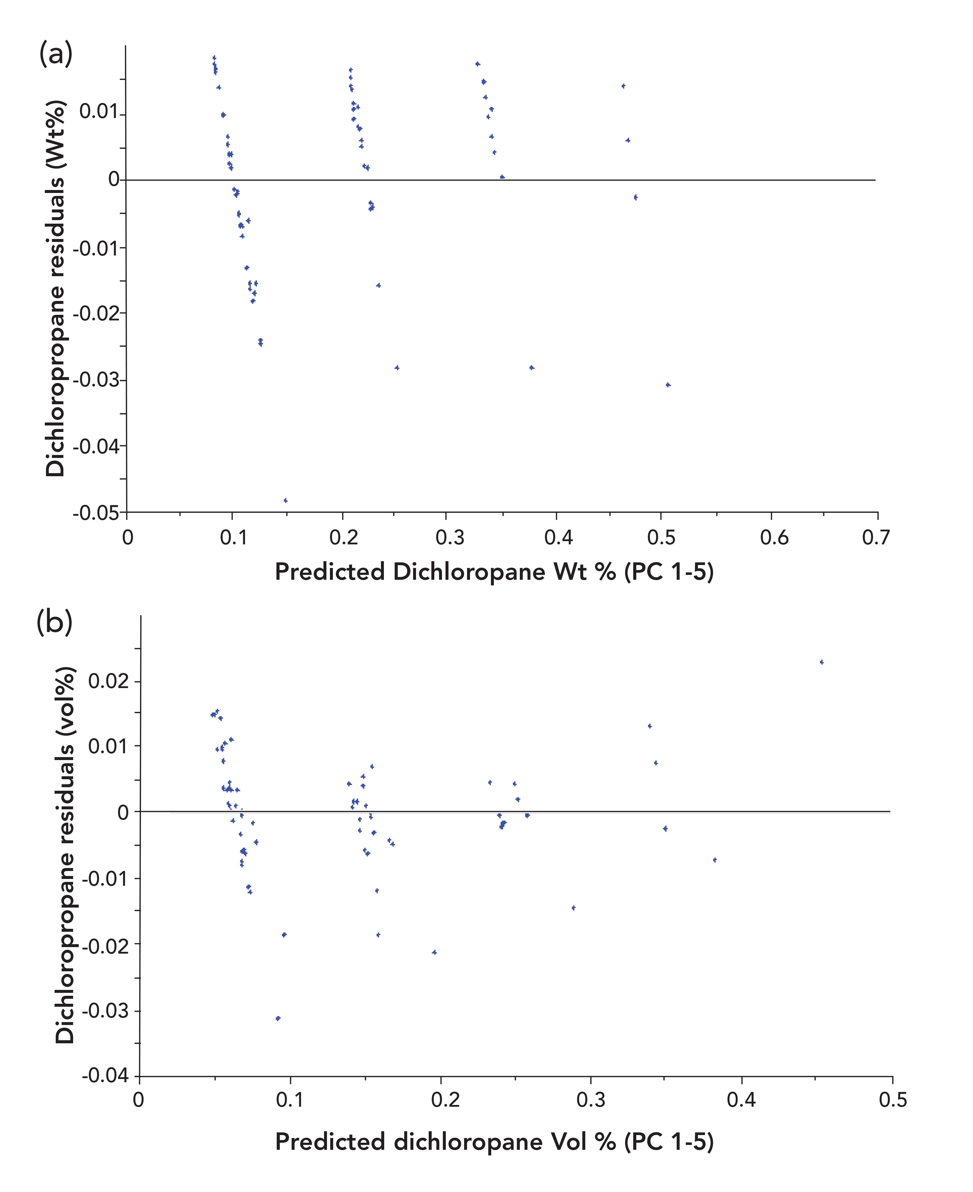
Direct plotting of the weight fraction and volume fraction plots against the PCR predicted values nearly erases the distinctions between the different cases; to the unaided eye, they all look like straight lines. It is possible to aid the eye by overlaying an actual straight line onto the graph. Then the difference between the weight fraction and volume fraction graphs can be observed, as can be seen from the plots on the CD, although we cannot include them here.
Conclusions
Our previous result (1) showed that the data do not conform to the theoretical expectations for the number of PCs needed to account for all of the spectral variance. This was a mystery until we saw the results reported here. Now we see that, because the PCs are computed solely from the spectral data, the use of different units for the constituent values cannot play a direct role in the need for those “extra” principal components that are computed. But figures 1 and 2 give us a clue as to the reasons why that happens nonetheless. In the absence of any prior information, we might expect that each PC would account for a more‑or‑less equal amount of variance from the spectrum of each constituent. Figures 1 and 2, however, show that is not the case. The first PC, for example, accounts for almost none of the acetone or butanol variance. The second PC accounts for almost none of the acetone or dichloropropane variance. We can see in Figure 1 that in several places, variance resulting from one or another particular PC is unaffected; several of these places are marked on the figure.
In the end, however, each of the constituents individually requires that four PCs contribute to the accommodation of the variance of that constituent and are therefore needed to remove all the variance from the data. Given, however, that for some constituents the early PCs do not reduce the variance, more than four total PCs are needed to explain the total variance of the data set. The conclusion previously ascribed (2) solely to the nonlinear relationship between spectroscopy and “concentration” expressed in incorrect units is now additionally seen to have another cause as well: It is a consequence of the direct relationship between the physical property (density) and mathematical properties (order of calculating PCs) of the spectroscopic data measured on samples affected by that physical property, and thus is only part of the explanation for the need for “extra” factors.
This finding is probably the most unexpected and surprising outcome from the analysis of this dataset. The finding that using the correct units for expressing concentration improves the analytical results and also makes the models more robust and reproducible is not nearly as dramatic, nor as much fun to use, as the application of increasingly complicated and sophisticated multisyllable chemometric methods. Nevertheless, being arrived at, and connected by a pure physical and chemical basis, it can improve the accuracy as well as our confidence in the results we obtain. Furthermore, contrary to our statement at the beginning of this subseries (1) about the state of near–infrared (NIR) spectroscopy analysis, we have now connected this field of endeavor to the rest of the universe of physical and chemical phenomena. There is still much to learn about the details, but now we can go in the right direction without being misled by the chemometric algorithms whose inner workings are impossible to understand.
Other Conclusions
Our study also yielded several other important conclusions that are worth highlighting. For example, even though the number of PCs needed to explain the variance introduced by the mixtures in the data set equals theoretically expected value, these are not necessarily the first n factors.
We also concluded the following for several chemical compounds: For the methanol results, there was a curvature seen on calibrations for weight%. We observed that it was masked by random variations at a low number of factors, and it was visible at a medium number of factors. The calibrations were reduced at a high number of factors and not observed on calibrations for volume%.
Meanwhile, for the dichloropropane results, we observed that the weight% exhibits a curvature at a low and high number of factors, and that the volume fraction shows no curvature at a low number of factors while reversing the curvature at a high number of factors, which “overcorrects” the non-linearity.
The PCR and PLS calibrations need the number (n) of factors expected from mathematical considerations. A possible explanation for the results is that the calibration algorithms reduce the random error contribution to the SEC but leaves the systematic error (such as the nonlinearity) relatively unaffected.
There were three regimes for operative changes to performance statistics: 1) Calibration corrects for actual changes in sample composition, 2) calibration accommodates itself to random noise, and 3) calibration accommodates itself to the nonlinearity of data.
Whether the effects 2 or 3 dominates depends on the data, and can change during the course of the calibration.
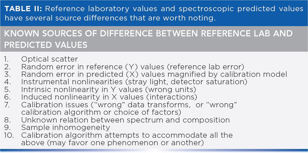
In addition to the above, we present here an expanded version of Table II from (1) listing the known sources of differences between the reference lab and predicted values.
References
- H. Mark, J. Workman, Spectroscopy 34(6), 16–24 (2019).
- H. Mark, R. Rubinovitz, D. Heaps, P. Gemperline, D. Dahm, and K. Dahm, Appl. Spect. 64(9), 995–1006 (2010).
Jerome Workman, Jr.serves on the Editorial Advisory Board of Spectroscopy and is the Senior Technical Editor for LCGC and Spectroscopy. He is also a Certified Core Adjunct Professor at U.S. National University in La Jolla, California. He was formerly the Executive Vice President of Research and Engineering for Unity Scientific and Process Sensors Corporation.

Howard Mark serves on the Editorial Advisory Board of Spectroscopy, and runs a consulting service, Mark Electronics, in Suffern, New York. Direct correspondence to: SpectroscopyEdit@mmhgroup.com
