Classical Least Squares, Part II: Mathematical Theory Continued

In our previous discussion, we based the computations on the condition that we knew the spectra of the pure components in the mixtures comprising the samples of interest. We continue our discussion of the theory by posing the question: What if we don't know the spectra of all the components in our mixtures, and (for whatever reason) cannot measure them?

Howard Mark

To answer this question, we again go back to equation 1:

and note the following: we started with the measured (and therefore known) absorbance for the mixture spectrum, represented by A, and the measured (and therefore known) absorbance spectrum of the pure material, represented by a. In this somewhat simplified presentation, the concentration of the analyte is calculated, from equation 13:

If we measured the spectrum of the pure component in the same cell as we are measuring the spectrum of the mixture, then we can form the equation:

where A_p is the absorbance of the pure material (which equals ab; when b is set to unity, the expression also equals unity).

Equation 1 represents the concentration of the pure material (that is, it's 100% pure material).

Jerome Workman

Dividing equation 13 by equation 14, we arrive at

A key point to note in equation 16 is that by measuring the spectrum of the pure material in the same cell we measured the spectrum of the mixture in, the pathlength of the cell dropped out of the equation (even if we hadn't previously set it to unity), and we are left with the fact that the concentration of the analyte is simply the ratio of the absorbance of the sample to the absorbance of the pure material.

The complicated-looking matrix equation shown as equation 12 (1) is in fact very similar to equation 16, it is simply the extension of this derivation to the case of multiple wavelengths, and the inclusion of the knowledge that the concentration of a given material is the same regardless of the wavelength we make the measurements at, so that we can use any or all wavelengths available for the computation.

Figure 1

For our current discussion, however, what's important is that of the three quantities in equation 16, two are known and one is unknown. Here, the two known quantities are a (the spectrum of the pure material) and A (the spectrum of the sample). This allowed us to solve for the third quantity, the concentration of the analyte.

Taking the same equation:

we now ask the same question as we asked at the beginning of this column: what if we don't know the spectrum of the pure analyte a?

That's OK. As we learned, again in our famous "high school algebra," as long as we know the values of all the other variables, we can calculate the one we want to know. In terms of equation 16 we can answer the question this way: if we solve equation 16 for a, the absorbance of the pure analyte:

We then note that if we measure the spectrum A of the analyte in the sample, and we also have the auxiliary information that specifies the concentration of the components in the sample, we can calculate a, the spectrum of the pure analyte. We could then use that spectrum as the spectrum to "plug into" equation 16 to use it to do future analyses in which we want to know the concentration, just as if we had measured the spectrum of the pure material directly.

Of course this is an idealization of the situation. In equations 16 and 17 we have assumed that the "spectrum" consists of the absorbance at a single wavelength, and we have also assumed that the analyte is the only absorbing component in the sample mixture.

To take into account the possibility of multiple absorbing components in a sample, we take another look at equation 2 (1), which includes the spectral contributions of multiple components:

Here, we cannot simply solve equation 2 for any of the unknown values of a, the absorbance of the pure materials. As we also learned in high-school algebra, when there are multiple unknowns in an equation, their values are undetermined because there are many (indeed, infinitely many) possible combinations of values that will produce the values A_j.

What to Do?

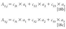
Here again we learned in high school algebra what to do. If we have some number of unknowns in our equation (let's say m unknowns; in equation 2, m = 3), then we need, as a minimum, that same number of equations, to be able to solve them and obtain a unique solution. Since, for example, there are three unknown quantities, a₁, a₂, and a₃ in equation 3, then we need two more equations, to create a set of three simultaneous equations that we need in order to be able to compute unique values for the absorptivities of those three pure materials. Therefore we first rewrite equation 2, and include as a subscript, the fact that this is the first of three equations:

We then add two more equations, representing the values corresponding to two more mixtures that might be used:

As general mathematical structures, these equations are satisfactory, but we also need to know how they relate to the problem we have set out for ourselves. Notice that a₁, a₂, and a₃ are the same in all three equations, as they must be if they represent the absorbances of pure materials. As we saw above, these are the unknowns in the simultaneous algebraic equations represented by equations 18, that are what we want to solve for.

The quantities a_1,j, a_2,j, and a_3,j are the total absorbances of three mixtures that we need to use for our data set. In general they will have different values, although under some special circumstances two, or even all three of them, may be the same.

The quantities c_i,j represent the concentrations of the three materials that comprise each of the three samples. As we saw in equation 18 and the subsequent discussion, along with the total absorbances of the mixtures, these concentrations are the algebraic "knowns" in the equations.

To solve the equations, the concentrations of the various components of the samples must have certain properties. In general, they must differ between the three samples. And while the concentrations need not all be orthogonal, it is extremely important they must not be linearly related, between any pair of samples, or between all three samples. For example, the concentrations of the components in sample 2 must not be a constant multiple of their concentrations in sample 1. We make the same requirement for the concentrations of components in samples 1 and 3, as well as for samples 2 and 3. Also, the sum (or difference) of the concentrations in one sample should not be the sum of their concentrations in the other two.

If all those conditions hold, then it is possible to solve equations 18a–c by ordinary algebraic means, and explicitly calculate the values of a₁, a₂, and a₃. It is not our purpose here, however, to illustrate the algebraic solution to simultaneous equations. Besides that we have all done that in high school, doing it in a spectroscopic context has also been illustrated in the context of the development of MLR ( in reference 2). What we will do here, though, is to quickly run through a simplified version of the mathematical development by transitioning from algebraic equations to their matrix representation. Equations 18a–c can be written in matrix form as:

where, as usual, the brackets indicate a matrix, and the symbols A, c, and a have the same interpretations as in the algebraic equation 3. Because in the matrix equation, as in the algebraic equation, A and c are the "known" values, we solve equation 10 for the unknown quantities, the spectra of the pure components, which are represented by [a] by first multiplying both sides of equation 10 by the inverse of matrix [c], that is, [c]^-1

Since any matrix multiplied by its inverse results in the unit matrix, we obtain

Equation 21 does not represent a least-squares solution, however. It is merely the result of solving simultaneous equations, and as is known from our previous work with MLR calibration, using the solution to simultaneous equations has some limitations. The chief limitation is the fact that the results are completely dependent upon the values used for the various individual numbers comprising [A] and [c]. Small errors in any of the data can have large effects on the results. The effects can be exacerbated if any of the data values are colinear, as we discussed earlier.

To reduce the effects of any of these problem issues, we proceed as we have done several times previously. We use more than the minimum number of required samples, and use least squares calculations to determine the values of the unknowns that minimize the (sums of squares of the) errors.

Table 1

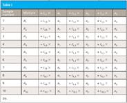
Here, we have known values for the absorbance of the mixtures and for the concentrations, and wish to solve for the absorbance of the pure components. We present these in Table I, for comparison with what we have seen previously.

As we see, the layout in Table I is the same as in our previous least square situations and therefore the least-squares development can be done similarly to the way it was done before, too. The only difference is that in Table I, the concentrations are different for each sample, while the absorbances are the constants of the equation, whose values are to be determined using least squares. Without going through all the gory mathematical details, we can note that we are trying to find values for the a_j, the absorbances of the pure-component spectra, that will allow us to best compute A_j, the absorbance of the mixture, for each sample. Becasue there is presumably some error in each measurement, we want to find the values of the a_i that provide the smallest sum of squares of the error in the computation of the A_j. Thus we compute e_j from the following expression:

We then follow the usual procedure of squaring the errors of each sample, summing the squared errors over all the samples, then taking the derivative of the sum with respect to the three (in this example) terms a_i, exactly the same way we did in reference 1, except using the appropriate data values.

When this is done, and converted to matrix expressions, the results are similar to those we found for the CLS computation when we know the spectra of the pure materials, and also to the expression for MLR calibration. We illustrate the comparison by rewriting the matrix equations below in Table II for comparison.

Table 2

Something we sort of swept under the rug, so to speak, is that all the earlier equations, from equation 17 to equation 22, refer to the values of absorbance (of samples and of pure materials) at a single wavelength. This is clear in equation 2, and perhaps even in some of the subsequent discussion. Once we get to equation 18, however, a reader might think that the multiple values of ai represent absorbances at different wavelengths, as is often the case in chemometrics applied to spectroscopy. Multiple absorbances in an equation are usually the absorbances of a substance at different wavelengths, this being the most common interpretation of "multivariate" in a spectroscopic context.

In this particular case, however, that's not so. The multivariate nature of the data in equations 18–22, as in Table II, are that the rows represent different samples, while the column represent, not different wavelengths, but different materials; the different materials are all measured at the same wavelength, for every sample. The differences in absorbance arise from the fact that different materials will, in general, have different absorptivities at any given wavelength.

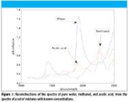
We demonstrate the application of this methodology in Figure 1, where, starting with a set of samples made from water, methanol, and acetic acid according to a mixture design (the details of which will be presented in a subsequent column) specifying 12 mixtures (and the three pure materials). The spectra of the 12 mixtures are used to compute the spectra of the pure materials, as specified by the equation in Table II; then these can be compared with the actual spectra of the pure materials.

The computation of the spectrum of the pure materials, therefore, arises out of the fact that we can apply equation 22 separately to each wavelength in the spectrum of interest. Computationally this might seems very inefficient, but in the computational form shown in Table II, the quantity [C^T ][CC^T ]^-1 need only be computed one time (because the concentrations don't change when you do the computation for a different wavelength), and so that matrix product need only be computed once and then multiplied by [A], the absorbance matrix for each mixture, to compute the values [a] of the various pure-material spectra at that wavelength.

Two caveats are needed for performing these calculations. The first caveat is how the "concentrations" should be expressed. While we will eventually have a lot more to say about the values that concentrations should be expressed in, for now, we will note that the concentrations should be expressed as fractions (or proportions) of the total, rather than percent, so that the sum of the concentrations of all the components in the sample equal unity, rather than 100%.

The second caveat is, in a sense, a result of the first caveat. If we perform a regression where, for every sample, the sum of the components add to a constant value (as in this case, where they all add to unity), we will quickly find that the matrix to be inverted ([CC^T ]^-1 ) is singular (that is, during the course of the computations a division by zero situation will be encountered). The way to deal with this situation is to eliminate one of the coefficients from the computations. The quick and dirty way (in other words, the wrong way) would be to eliminate one of the concentrations from the set of equations. However, that is, as stated, the "wrong" say because it would then ignore the contribution of that sample component to the calculations. The right way to do the calculation is to eliminate the constant term (a₀) from the computations. Draper and Smith (3) demonstrate (on p. 412) how the regression equations need to be modified to accommodate this calculation.

Figure 1 shows that reasonable representations of the pure component spectra are obtained by this means. A more critical view of the spectra can be obtained by comparing them to the original, measured, pure component spectra, which we do in Figure 2. The three parts of Figure 2 show the comparisons of the reproduced spectra with the original measured pure water, methanol and acetic acid spectra. We see that, as with the reproduction of mixture spectra in part I of this column, while the reproductions are "about right," a more critical look at the comparison reveals appreciable flaws in the results. In particular, we see that the calculated methanol spectrum in Figure 2b has a peak at roughly 1940 nm, corresponding to the water peak at that wavelength, as does the calculated acetic acid spectrum, neither of the actual spectra have that peak.

Figure 2

While the mathematics of CLS calibration is not inherently more difficult than the development of some of the other, more common, calibration methods, it is rarely used in modern chemometric practice. The reasons for this are not theoretical, but practical. While the equations derived are straightforward enough, they are derived for those situations to which Beer's law strictly applies — that is, clear (that is, nonscattering) liquid solutions.

This is the first stumbling block in the application of the CLS method; most current applications of chemometric analysis are for powdered solids, or, even if liquids are of interest, they are often emulsions, gels, or some other type of scattering sample.

Even in those cases in which clear liquid mixtures might be of interest, there are other difficulties. The first difficulty is that it might not be possible to obtain or measure the spectrum of all the components of the mixture. As in applications in which other calibration algorithms are commonly used, as for example, with natural products, it might not be possible to extract every component and measure its spectrum. Indeed, in complicated samples, not all the components might be known, much less methods to extract them; of course, any extraction method, to be useful, must not degrade the component or change its spectrum.

In many cases, the spectrum of a pure component, after being extracted from the sample, is not the same as the spectrum of that component in its natural state in the sample. This caveat is critical even in what might be thought of as a "simple" case, that of water. A notorious example of this is water in many natural products, where the interactions with the surrounding materials changes the spectrum of the water compared to its spectrum in the pure state. Water is by no means unique in this respect.

Earlier in this column, we showed how to deal with those samples where the pure-component spectra are unknown, so a natural question to ask at this point is why not apply that concept, and determine the pure-component spectra from a set of mixtures?

We could indeed do that. The necessary procedure would be to obtain a suitable set of samples, measure their spectra, and measure, using wet chemistry or another laboratory (in other words, reference) method, the concentrations of all the components. However, why do this, when the MLR algorithm has the same requirements except that only the concentration of the analyte needs to be measured using a reference laboratory?

Basically, to use CLS for this purpose would have all the requirements of MLR "on steroids" so to speak. Again, this is a matter of practicality, rather than any inherent defect of the CLS method itself.

A more serious reason for not doing that is revealed by the results from this demonstration of the CLS method: the relatively poor reconstructions of the target spectra; this constitutes a more significant drawback to the method. Between the two drawbacks, therefore, the CLS approach is rarely used.

In our next column, we will examine the discrepancies between the measured and reconstructed spectra that we saw in both columns in more detail, and the causes of those discrepancies. We also will look at the behavior of the CLS algorithm in more detail, to see how what we've learned can be applied to obtain useful results.

Howard Mark serves on the Editorial Advisory Board of Spectroscopy and runs a consulting service, Mark Electronics (Suffern, NY). He can be reached via e-mail: hlmark@prodigy.net

Jerome Workman, Jr. serves on the Editorial Advisory Board of Spectroscopy and is currently working in the medical device industry using spectroscopy. His email address is: JWorkman04@gsb.columbia.edu

References

(1) H. Mark and J. Workman, Spectroscopy25 (5), 16–21 (2010).

(2) H. Mark, Principles and Practice of Spectroscopic Calibration (John Wiley & Sons; Hoboken, New Jersey, 1991).

(3) N. Drape and H. Smith, Applied Regression Analysis, 3d ed. (John Wiley & Sons; Hoboken, New Jersey, 1998).