Combining Broadband Spectra and Machine Learning to Derive Material Properties

A quiet but interesting trend has been occurring in material analysis, coincident with the rise of artificial intelligence (AI) and so-called "deep" machine learning methods. Astute spectroscopists have always known that there is more information in the spectra that they obtain than simply the molecular or atomic peaks that are directly measured. Particularly with methods such as infrared, Raman, and laser-induced breakdown spectroscopy (LIBS), the spectral background contains a wealth of information about the sample, and analytical combinations of the peaks can provide material properties. Traditionally, such analytical combinations of peaks were performed explicitly by analysts, but now information about material properties embedded in the spectra can be derived implicitly by AI and machine learning algorithms. This column introduces these ideas and touches on recent results indicative of what more may be coming in this direction.

Computer calibration and learning technologies go by a variety of different names, depending as much on the application as on the algorithms used. Machine learning in its broadest sense refers to the automation of learning without an explicit program, and is used for everything from image recognition and voice recognition to stock selection. In many cases, the machine-learning algorithm is selected with some knowledge of the mathematical characteristics of the problem to assist in performance. Deep learning refers to the subset of machine leaning that uses a model learning representation rather than a task-specific algorithm. An example of deep learning could be a neural network or other biological model. Chemometrics usually refers to multivariate statistics and machine-learning algorithms applied to chemical and biological systems to extract information. Finally, artificial intelligence (AI) may be described as machine intelligence, the expression of some problem solving or learning ability (typically in a narrow area) that humans would equate with cognition. The best-known recent example of AI may be IBM's Watson computer, which has beaten chess grandmasters and reigning champions on the popular game show Jeopardy.

When we make the shift from traditional methods of calibration and analysis to chemometrics, we gain power at the expense of complexity and opaqueness of the model. Previously, to use an atomic spectroscopy example, if we were to build a calibration for chromium in an arc-spark spectroscopy system, we would find a promising emission line that varied predictably over the required range. We would measure the integrated intensity of that background-subtracted Cr emission line over the range, and build a calibration curve that allows prediction of the Cr concentration from the strength of the emission line. Multivariate methods such as partial least squares (PLS) regression or principal components regression build the calibration curve using multiple input variables, which may be positively or negatively correlated with the element being predicted. Extending our chromium example, multiple lines of Cr would be positively correlated with the concentration of Cr in a prediction. In the case of a stainless steel, which may have chromium concentrations of 1–20%, iron concentration may actually vary inversely with Cr concentration. We would then see a negative correlation between Fe emission lines and Cr concentration that could be used in a multivariate model. Using these algorithms we can easily back out specific relationships (negative or positive correlations) in the regression model corresponding to each input.

Increasing in complexity and opaqueness, examples of ensemble learning include support vector machine (SVM) and random forest methods for classification and regression. These methods use large quantities of labeled (or quantified) training data to build predictions. In SVM, data are projected into a new coordinate system such that dividing hyperplanes can be used to build categories or regression steps in the data. In random forests, many decision trees are built during classification using subsets of the data, and the classification or regression answer is found by selecting the most frequent (mode) of the prediction. Both of these methods are well-suited to complex, nonlinear problems. However, after a prediction is made, it is nearly impossible to get "inside" the algorithm to determine the relationship between a specific input variable and the prediction, short of a Monte Carlo–type simulation.

Finally, artificial neural networks (ANNs) mimic animal brains, with connections between different neuronal layers doing the processing. One of the first types of AI, pioneered in the 1950s, it has only been in recent years that the power of ANNs could be fully exploited as sufficiently powerful computational resources have been developed. In an ANN, a number of inputs (which could be points in a spectrum) are input. Each input is sent separately to nodes in a "hidden layer." At the hidden layer, the inputs are combined, using weights for each input that are determined by training. The outputs of the hidden layer may go directly to the output of the model (prediction), or to a second, and third hidden layer, and so on, before the output. The structure of the network between the hidden layers and the method of determining the weightings can also be variable. Similar to the SVM and random forest, it is difficult if not impossible to unpack the "training" of an ANN into logical steps.

Examples

Recently, researchers have used tools ranging from multivariate methods to ANNs to solve complex spectroscopic problems involving material properties. Here, we explore a few examples that point to how this is accomplished in practice.

Raman and Infrared Spectra Determine Diesel Fuel Properties

Diesel fuel is not uniform, but in the case of petroleum-derived diesel, it typically comprises carbon chains between 8 and 21 carbon atoms in length. Diesel can also be derived from biomass, coal liquefaction, and even animal sources. Given the variety of sources, property measurement is important because no standard formulation exists. In blending diesel fuel, properties such as viscosity, density, and ignition characteristics are key parameters. Viscosity and density determine the flow rate at a given manifold pressure through the injectors, and influence the droplet size and dispersion, related to the spray characteristics. The ignition characteristics are measured through the cetane number (CN), which is a measure of the compression-ignition characteristic of the fuel. The higher the CN, the faster the combustion and the lower on the temperature–pressure curve the fuel will ignite. Cetane (hexadecane) is easy to ignite and is given the arbitrary number of 100, while typical diesel fuel in the United States has a cetane number between 40 and 55.

The measurement of density is simple, the measurement of viscosity is only slightly harder, but the measurement of CN is actually quite involved. Originally, the fuel in question had to be burned in a special test engine while varying the compression ratio of the engine to achieve a specific ignition delay. From this data, the CN could be calculated. A simpler fuel ignition tester is now used to determine ignition delay and thus the CN, but it still requires a combustion measurement.

Bolanča and coworkers decided to use Fourier transform-infrared–attenuated total reflection (FT-IR-ATR) and FT-Raman spectra of fuels combined with artificial neural networks to try to predict these fuel properties (1). For both methods, spectra included both the fundamental C-H stretch region and the fingerprint region, because the spectra were roughly in the 500–4000 cm^-1 range. Typical spectra are shown in Figure 1.

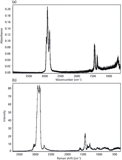
Figure 1: Typical spectra of diesel fuels: (a) FT-IR-ATR, (b) FT-Raman. Adapted with permission from reference 1, under the Budapest Open Access Initiative.

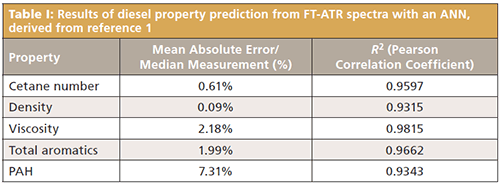
These researchers found that, in general, both FT-ATR and FT-Raman methods were able to predict properties with an accuracy approximately equivalent to the uncertainty of the standard test methods, when the 45 samples in the training set were fed into an artificial neural net with a multilayer perceptron model and eight hidden layers. For everything except polycyclic aromatic hydrocarbon (PAH) prediction, the FT-ATR data performed slightly better than the FT-Raman data. Table I shows the results of the best-performing model with the FT-ATR data as shown in Figure 1a.

Determination of Coal Properties Using Laser-Induced Breakdown Spectroscopy

As a naturally occurring, relatively unrefined fuel, coal exhibits a wide range in the properties that are most important for combustion. The primary properties of coal measured in a "proximate" analysis include the heating value (MJ/kg), volatile matter (%), fixed carbon (%), and ash (%), among others. Standard laboratory measurements exist for each of these crucial parameters; typical analysis may take 6 h or more to complete. It would be useful to have a real-time, or nearly real-time, analysis method that could be used for sorting coal by quality at the mine site, blending coal efficiently, spot-checking coal quality for transactions, and control of coal firing in boilers. In particular, more efficient coal firing could help reduce particulate matter and greenhouse gas pollution from coal utilization.

Wang and colleagues at Tsinghua University have published several papers on coal property determination from laser-induced breakdown spectroscopy (LIBS) spectra using a modified "dominant factor" PLS method. The most recent paper (2) describes a spectral normalization method designed to remove the shot-to-shot fluctuation from individual LIBS spectra taken on the same sample, which can be caused by local material changes or laser fluctuations, which affect ablation efficiency and electron density in the plasma. Following spectral normalization to obtain a "standardized" spectrum, a subset of lines known to be physically related to the desired quantity (called the dominant factors) is used in an initial PLS prediction to estimate the property in question. An example of dominant factors might be elemental emission lines associated with minerals for prediction of ash percentage. In training, the dominant factor PLS estimate, which is much more accurate than typical PLS with the entire spectrum, is compared with the known quantity. The entire spectrum is fed into a secondary PLS to determine a "correction" signal, so that the trained algorithm uses both a PLS based on the dominant factors and on the entire LIBS spectrum to arrive at a property prediction. In this case, after a prediction is made the result is stored in a database so that if the same sample is encountered again, it can be recalled, significantly reducing shot-to-shot variation on the same sample.

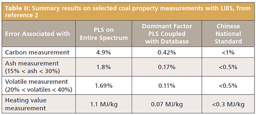
Figure 2 illustrates prediction of volatile matter in coal using the dominant factor PLS model. Like the heating value, volatile matter is one of the coal properties that is more unrelated to the individual elements. Most volatile matter is made up of carbon and hydrogen atoms, but these can also be found in fixed forms in the coal. Hence the chemometric algorithm needs to do the heavy lifting to find the patterns in the spectrum that correspond to volatile versus fixed forms of hydrocarbons. In Figure 2, the black triangles show the calibration data, and the blue and red symbols show the validation data. For all of the properties mentioned, selected summary results are shown in Table II, compared with PLS on the entire spectrum and compared to the Chinese National Standard for coal measurements.

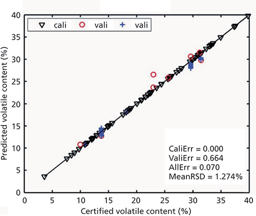
Figure 2: Calibration and prediction of volatile matter in 77 coal samples. Adapted from reference 2 with permission from the Royal Society of Chemistry.

Measurement of Jet Fuel Properties in the Near Infrared

Given the requirements for safety, jet fuel is under rigorous specifications for properties such as flash point, freezing point, and boiling point, which are surrogates that indicate the combustion properties of the fuel. These properties may slowly change over time, as well as by batch of fuel received or by contamination. Therefore, rapid measurement of these properties is useful. Xu and colleagues conducted a near-infrared (NIR) study of jet fuels (3) comparing a standard partial least squares-discriminant analysis (PLS-DA) method to a fuzzy rule-building expert system (FuRES) (4) and a support vector machine (SVM). The FuRES is a type of minimal neural network architecture. The SVM and the FuRES had similar performance, significantly better than the PLS-DA method.

The sample set consisted of 49 samples of jet fuel sampled in triplicate. The goal was to classify the previously mentioned temperature properties into "low," "medium," and "high" ranges. Table III illustrates the prediction accuracies for these fuel properties.

Implications

The writing on the wall is clear. As computing power and memory continue to increase, we should be thinking about how to generate enough of the right kinds of data to feed machine learning algorithms. PLS and principal components analysis, which are widely used, only scratch the surface of what is possible. Algorithms that are better able to handle nonlinear, multifactor data such as SVM or random forests may prove useful. Genetic optimization and Bayesian inference also may reveal a lot in the data, and allow us to experiment more efficiently and converge more quickly on an answer. As spectroscopists, we should be learning the pluses and minuses of each of the key methods of machine learning, or at least making friends with the data scientists, so that we can get the most out of our data. There is a wealth of great references, with one of the most engaging entrees to machine learning being Pedro Domingo's The Master Algorithm, which clearly explains the various branches of machine learning, their strengths, and the search for combinations of learning algorithms to enhance AI overall (5).

Data quality is still paramount. No amount of computer processing can yield great results from nonexistent or poorly acquired data. However, it is true that properly applied algorithms can sometimes pull a rabbit out of the hat, or the signal from the noise. As we have tried to indicate here, machine learning methods can often pull surprising macro properties out of spectra that we would have suspected of only having elemental and molecular data in the past. The key thing for training such algorithms is good quality data, and often lots of it taken over time.

Several years ago, Google started a focused effort to train image recognition to recognize cats from the millions upon millions of cat (and non-cat) images on its search engine. Now Google's image search can equal or outperform a human in many image recognition tasks. Deep learning algorithms can outperform pathologists in detecting some cancers, and Microsoft Research announced in August that its algorithms can equal or surpass human translators on the classic "Switchboard" conversational speech recognition task, transcribing real conversations. All of these tasks involve massive amounts of training and computational data at the outset, but once the model is made the task becomes automated and easy.

As spectroscopists, we are good at getting quality data. We should be asking ourselves which problems would benefit from machine learning, and elevating our game thereby. As these examples show, it is likely that we can push the boundaries-measuring new properties and detecting new things-by harnessing the power of AI.

References

(1) T. Bolanca, S. Marinovic, Š. Ukic, A. Jukic, and V. Rukavina, Acta Chim. Slov. 59, 249–257 (2012).

(2) Z. Hou, Z. Wang, T. Yuan, J. Liu, Z. Li, and W. Ni, J. Anal. At. Spectrom. 31(3), 722–736 (2016).

(3) Z. Xu, C.E. Bunker, and P.d.B. Harrington, Appl. Spectrosc. 64(11), 1251–1258 (2010).

(4) P.d.B. Harrington, J. Chemom . 5(5), 467–486 (1991).

(5) P. Domingos, The Master Algorithm (Basic Books, New York, 2015), pp. 329.

Steve Buckley, PhD

Steve Buckley, PhD, is the CEO of Flash Photonics, Inc., an affiliate Associate Professor at the University of Washington, and a consultant to the spectroscopy industry. Direct correspondence to: SpectroscopyEdit@ubm.com