More About CLS, Part 1: Expanding the Concept

This column is the first of a set that expands our previous discussions of the classical least squares (CLS) algorithm. Having found a new effect that can introduce a large error in calibration results, we extend our investigation of the effects of this phenomenon to calibrations using principal component regression (PCR) and partial least squares (PLS) that we were previously unable to do. 

A while back, we published a series of columns, and a formal paper, about classical least squares (CLS) analysis of liquid mixtures (1–15) to deal with and explain the use and behavior of CLS analysis for calibration. We review and summarize here what we found from the results of those columns, preparatory to analyzing a similar but more extensive experiment.

That all started out from a very modest goal: to explain CLS analysis of spectra, and the relationship of the CLS mathematics to the mathematics used for multiple linear regression (MLR) applied to determination of the composition of mixtures. We also wanted to further demonstrate the application of the CLS approach to determining the composition of some simple liquid mixtures. Along the way, we discovered some unexpected relationships between the spectral measurements and the chemical composition, which we explored in those columns.

However, along with the discovery of the unexpected effects, we also gained insight into many previously known, but unexplained, phenomena that have been afflicting spectroscopic analysis since time immemorial. Since the beginnings of modern near-infrared (NIR) analysis, there have been many symptoms of problems that are known to affect our ability to find the relationship between the spectral data and the sample composition, but nobody had been able to definitively pin down the causes of those symptoms. Hence, in our own minds we have considered these as "mysteries" of spectroscopic analysis. Table I presents a list of these mysteries. Much of this column is based on a presentation at the Eastern Analytical Symposium in 2013 (20).

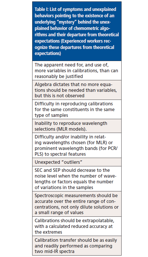
These mysteries, and confusion over them, have existed since the beginnings of modern NIR analysis. Indeed, when one of this article's authors (HM) first joined Technicon Instruments in 1976 (one of the first commercial companies to manufacture NIR spectrometers to address the requirements of this new analytical method based on Karl Norris's pioneering work), he found the same questions were already being asked by the engineers and scientists at that company, questions that have persisted until recently. Other newcomers to the company would also say things like, "I studied and thought I knew spectroscopy and how it's used, but here we have no baselines, no standards, no pure-component spectra, no a priori theory, and no spectral interpretation. But it works!" Indeed, not having explanations at that time for the effects seen made NIR analysis appear to be divorced from the mainstream of spectroscopy, and existing in a universe of its own separated from the universe of the rest of science.

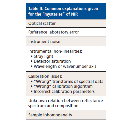
The general NIR community, which at that time was very small, shared the confusion over the behavior of NIR data. Attempts to explain this anomalous behavior went on for many years. Several of the common explanations that were proposed are listed in Table II. Some of those common explanations have within them subcategories. For example, use of the "wrong" calibration algorithm has, along with it, the use of an incorrect number of factors (for the principal component regression [PCR] or partial least squares [PLS] algorithm), or the wrong number of wavelengths (for the MLR algorithm). The use of MLR also carries with it the possibility of using the "wrong" wavelengths (even if the number of wavelengths is correct). Note that the equivalent is also true; for example, for PCR or PLS. However, that possibility usually goes unrecognized and unnoted, because most of the software packages available do not allow the user to select arbitrary subsets of the factors computed during the execution of the PCR or PLS algorithm. For example, a user who decides to create a model that uses four principal components (PCs) is generally not free to select which four components to use; with all the software packages for spectroscopic analysis we're familiar with, only the first four PCs may be used. This limitation is both a curse, and a blessing. The curse is that the limitation prevents users from selecting just the minimum number of factors needed to optimally analyze the samples of interest. If, for example, the sixth factor is important, the user cannot select four factors that include the sixth, but are forced to include extra, unnecessary factors, such as the third and fifth, perhaps, that contribute to overfitting. The blessing is that most users are already confused by complicated algorithms they are not comfortable dealing with, and are happy to not have another whole set of choices to make.

Over the years, many scientists have tried to address one or more of the suspected problems. The approach usually consisted of hypothesizing a cause of the problem, and then taking an empirical approach by applying an ad hoc solution, usually as part of the routine chemometric algorithm in use. Surprisingly, often this approach "worked," insofar as the scientist was able to obtain satisfactory calibration and prediction performance for the analyte of interest in his samples, and assumed that his "fix" was actually correcting the situation. On the other hand, even when that was the case, this approach usually gave little insight into the underlying causes of the difficulties encountered. Even worse, the results obtained could rarely be generalized or extended to other applications of NIR, or for other types of analysis.

As described above, around 2009–2010, with the assistance of colleagues, we performed some experiments that we expected would shed some light on the subject (15). The goal was to physically remove as many of the suspected error sources as could be managed. Therefore, samples were made up as binary and ternary mixtures of clear liquids (dichloromethane, toluene, n-heptane). These materials were all mutually soluble in all proportions, and had well-defined and distinct spectra. The use of clear liquids removed any possible difficulties due to optical scatter in the samples. Making up the samples gravimetrically removed the "reference lab errors" usually encountered when performing routine NIR calibrations, since no "reference lab analysis" was performed, and the sample compositions were known as accurately as the weighing technology used. An experimental mixture design specifying 15 ternary samples, each sample containing the three completely miscible organic liquids, was generated and analyzed. The design contained mixtures at evenly spaced concentration (by weight) levels, going from 0 to 100% of each of the three components. The experimental design is described in reference 5.

Spectra of all 15 samples were measured in transmission, and Beer's law holds. This experiment used is, therefore, the simplest one we could think of that covers the full range of all components and binary and ternary mixtures. Similarly, the data analysis applied to the spectral data was the simplest data analysis we could think of: We used the CLS algorithm, and applied it to the spectral data without any mathematical pretreatments. This was also described in the previous columns (2,16). The use of the CLS algorithm does impose some requirements on the data:

• Spectra of the pure raw materials must be known.

• There must be no interactions that affect the spectra, between the mixture components.

• There must be no partial molal volume effects.

As long as the conditions are met, this experiment constituted the simplest spectroscopic system for applying chemometric algorithms. The results showed that there was nonlinearity in the relationship between the spectroscopic measurements and the reference values for concentration when the reference values were expressed as weight percent (or weight fractions), as is common practice for many NIR analytical methods of interest.

However, the relationship between the spectroscopic measurements and the reference values for concentration was found to be linear when the reference values were expressed as volume fractions. The underlying root cause turned out to be grounded not in the spectroscopy, but in the very straightforward and elementary physical chemistry involved: When liquids of different densities are mixed, the weight fraction and volume fraction of any given component of the mixture are not the same. These relationships are shown in Figure 1, for the three-component mixtures used for the experiments we described above. Another effect, well known to physicists, but apparently not so well known to chemists and spectroscopists, is that light interacts with matter in proportion to the volume the matter occupies (full disclosure here: We did, in fact, recently come across a rare exception noted in a recent article that used volume fractions when specifying interactions of light with matter, but that was not in the context of performing analysis [19]). Thus from the physical theory of absorption as well as the experimental results, we find that it is the volume fraction of the mixture components that determines the Beer's law absorbance.

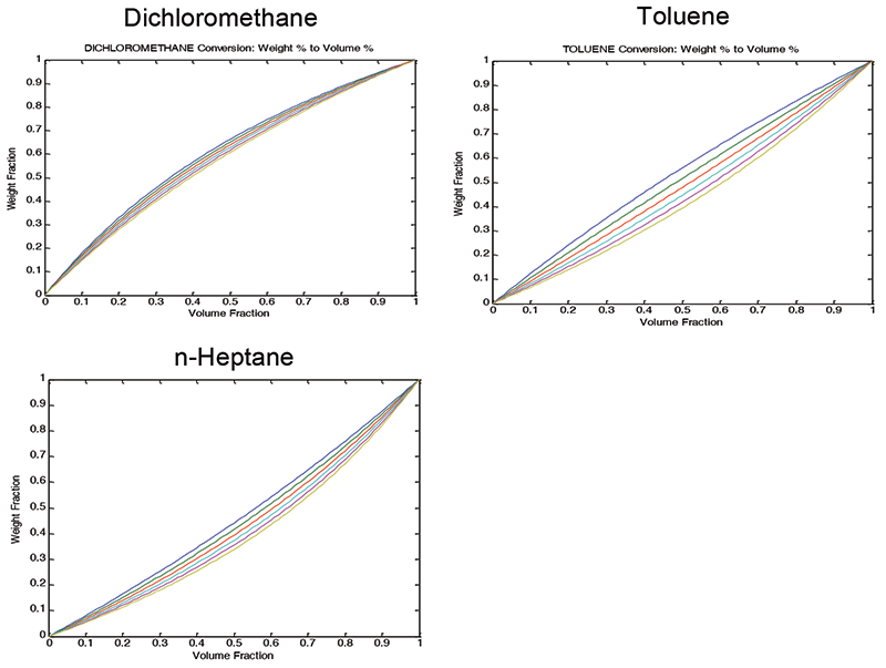
Figure 1: Underlying cause of nonlinearity: weight fraction (y-axis) versus volume fraction (x-axis) ternary mixtures containing toluene, n-heptane and dichloromethane exhibit non-linearity between weight fraction and volume fraction as measures of concentration of the components. The heading of each graph indicates which constituent is having its weight-versus-volume fraction plotted. Each graph contains a family of curves, due to the changing relative amounts of the other two constituents.

Because the volume fraction is the "concentration" measure that is linearly related to the spectral measurements, it is clear that any other measure of concentration that is nonlinearly related to the volume fraction must also be nonlinearly related to the spectroscopic values.

These results were also published in an Applied Spectroscopy article (15). Figure 1 shows how the continuum of values exhibits the curvature. Plotting residuals is a time-honored way to gain the ability to examine calibration results more closely than the straight forward x-y plot allows. By preventing the range of the data from filling up the y scale in favor of the residuals which then expand the errors to fill the scale, this way of plotting data allows the analyst to look at the data through what amounts to a digital "magnifying glass," thereby seeing aspects of the data that are hidden in the standard X-Y plot. Figure 2 displays the result of plotting residuals of the data, instead of the raw data, on the ordinate. It is obvious how the plot becomes expanded.

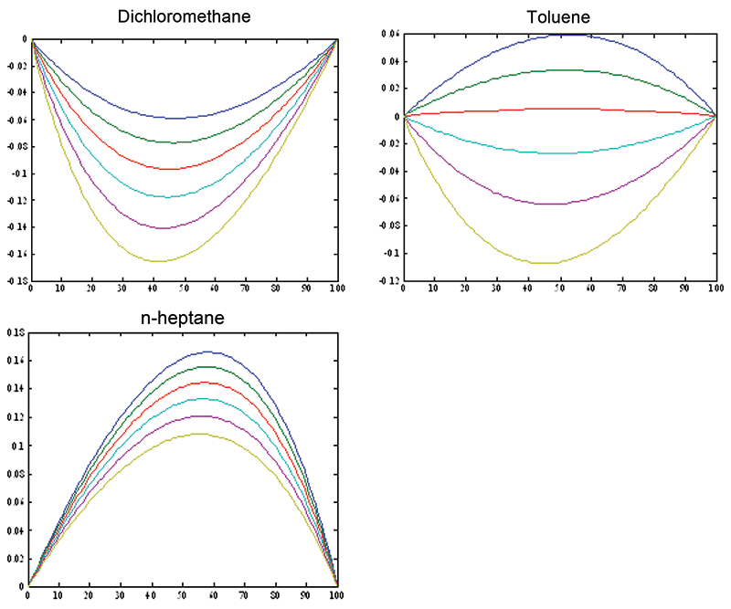
Figure 2: Residuals: differences between the volume percent values (x-axis) predicted by the model, minus the actual weight percent values (y-axis). This type of plot expands the differences for closer scrutiny, by plotting these residuals instead of the raw ordinate data (as in Figure 1). By removing the range of the data from the y-axis, plotting residuals allows us to put a "magnifying glass" on the behavior of the data. This expands the differences for more careful study. Note that these plots are schematic, to show the effect of non-linearity between weight-based and volume-based units. The effect on representative data will be illustrated in Figure 4.

The continuous curves are useful for displaying the underlying nonlinearities that the data are subjected to. Ordinarily, however, actual samples do not display a continuum of values. In the most common scenario representing analytical procedures, samples are selected at random, and therefore contain, and represent, some random selection of concentrations of incidental ingredients as well as of the analyte. This random selection of samples, in our hypothetical case, therefore contains a quasi random sample of the three-component mixtures represented by Figure 1. This random selection is shown in Figure 3, where the round dots, representing the actually selected samples, are displayed simultaneously with the continuum. However, the points all lie so close to the continuum, and to each other, that it's difficult at best to see anything else that might be in this data plot.

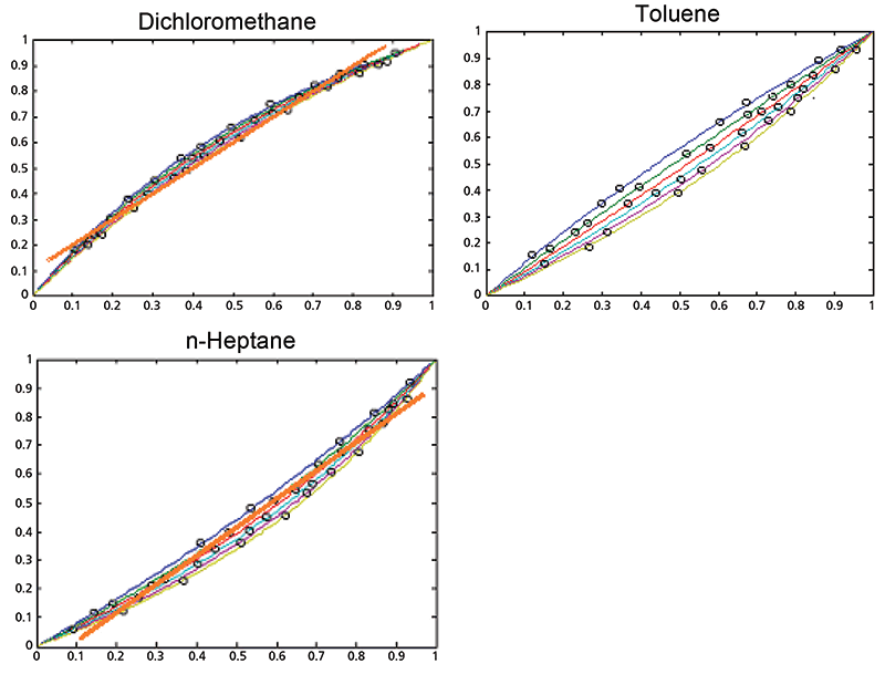
Figure 3: Underlying cause: weight fraction (y-axis) versus volume fraction (x-axis), showing the effect of random sample selection, overlaid with an actual straight line. The black circles on each plot represent the random samples that might have been taken from the underlying continuum of mixtures. When samples are selected at random, you don't see the underlying curvature. The error values seem randomly scattered around the average curve, just as though the error was random instead of systematic, as a result of the random sample selection. A calibration, however, will show curvature in the residuals.

When samples are selected at random, therefore, you don't see the continuum or the underlying curvature, because the random selection of samples only allow randomly distributed data points to be displayed on the plot. The error values appear randomly scattered around the average curve, just as if the error, despite being completely systematic, were itself random, due to the random sample selection. This is demonstrated in Figure 3. Although Figures 3 and 4 are schematic, the plotted points in Figure 3 illustrate how the points tend to cluster around the calibration line, but the range of values of the data makes it difficult to see the departures from linearity. Figure 4, showing the residuals from the data of Figure 3, again shows how plotting the residuals applies a digital "magnifying glass" to the results of Figure 3. A calibration containing nonlinearity will, therefore, show curvature in the residuals, which might not show up in a plot like Figure 3. This is demonstrated in Figure 4, where the residuals are again plotted on the ordinate instead of the raw ordinate values. This method of inspecting the results not only shows up nonlinearity, but also enables observing any clustering of data, as well as other potential fault conditions to be displayed for the user's inspection. When we look at actual data, we will see how this new tool can be helpful in finding out what is going on "under the hood" of the data analysis.

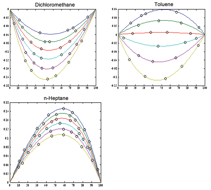
Figure 4: Plot of the residuals from Figure 3, as the differences between the volume percent values (x-axis) minus the actual weight percent values (y-axis). This type of plot magnifies the differences and allows more sensitive detection of the non-linearity. Note that these plots are schematic, to compare the effects of using volume-based units to weight-based units. The continuum of values from which individual samples' values are taken is shown for comparison, as per Figure 2.

To be sure, this new finding that the volume fraction is the correct analytical quantity to use for calibration does not automatically solve all problems with NIR calibrations. A chain is only as strong as its weakest link. Finding a new "weak link" does not eliminate the possibility of one or more of the classic potential problems plaguing our efforts to create calibrations, listed in Table II, from entering and creating difficulties in the calibration process. But it is one more item to consider when problems arise, and a good scientist wants to understand an analytical system instead of blindly applying "brute force" chemometrics to cover the problem up.

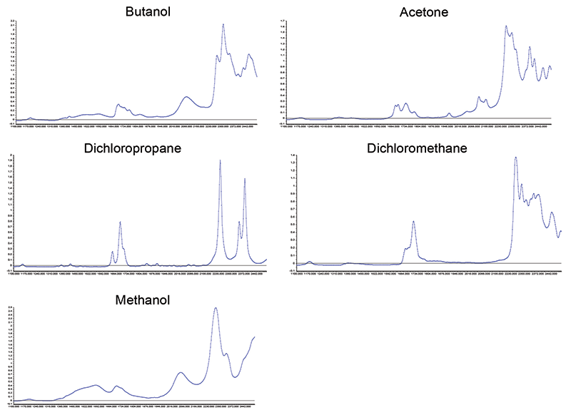
Figure 5: NIR spectra of the five pure constituents in the expanded set of mixtures. X-axis is wavelength (in nm) and y-axis is absorbance.

Expanding Beyond the Small Dataset

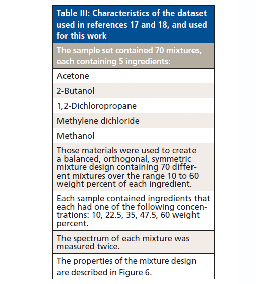
The foregoing makes a compelling case that, for spectroscopic analysis, EM radiation "sees" the absorbance according to the volume fractions of their components (given some assumptions to ensure ideality, or near ideality). Physical theory tells us that this is what we should expect, and we find that the CLS algorithm is responding according to the theory. This does not automatically ensure that conventional calibration algorithms will respond the same way, and a strictly scientific approach requires that we verify that the performance of the calibration algorithms are evaluated by actually applying them to the set of data. The fifteen samples' worth of data we had available, and used for this study, is not sufficiently large to reliably test the conventional calibration algorithms. A search for another, larger, suitable sample led us to a pair of reports, by Willem Windig and colleagues, based on data suitable for our purposes (17,18). With the assistance of Tony Davies and Tormod Naes, Prof. Windig was contacted and graciously offered to supply the data used for his studies. The dataset contained spectra of mixtures of five ingredients: acetone, 2-butanol, 1,2 dichloropropane, methanol, and methylene dichloride. In addition to the mixtures, the spectra of the pure components had also been measured, and are part of the set. This dataset is not perfect; the presence of two different alcohols may lead to potential interactions. There may also be interactions caused by the two chlorine (Cl)-containing polar materials in the set, but the design is completely symmetric and balanced, and is otherwise a nearly ideal set of mixture spectra. All samples specified by the design were made up and scanned twice. Examination of the scans revealed that plots of the two repeat scans from any sample were indistinguishable by eye on the computer's monitor.

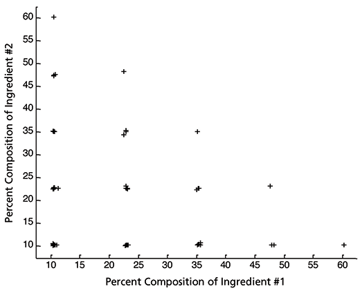
Figure 6: Overall characteristics of the orthogonal, balanced, symmetric statistical experimental design used to define the samples. The five different ingredients allow for ten pair wise comparisons; each of the ten possibilities provides a plot that looks like the one presented below. Any and all pairs of ingredients, when their percentage composition is plotted on an x-y plot, generate this pattern.

The characteristics of the dataset are described in Table III. For reference, the spectra of the pure ingredients are shown in Figure 5. There were two spectra measured for each pure ingredient; when plotted together, as in Figure 5, we see that the two spectra completely overlap, indicating that spectral noise or other source of variation is negligible.

Because there are five ingredients, there are 10 combinations of ingredients that can be plotted pairwise. The experimental design is such that any and all pairs of ingredients, when plotted on a x-y plot, generates a pattern like the one shown in Figure 6. The method of generating the design is described by Windig (17,18).

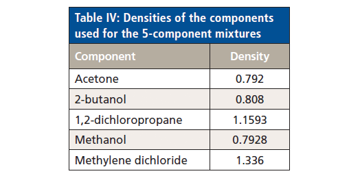
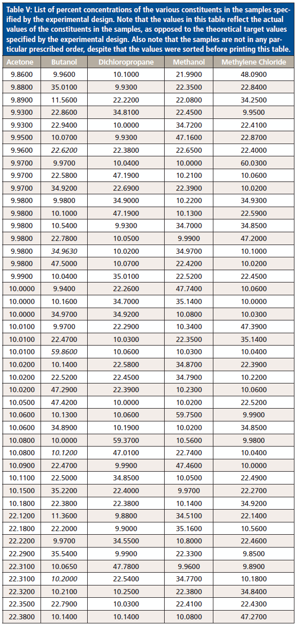
Because we want to observe the effects of using both weight fractions and volume fractions as the component concentrations, we used the values for density of the various compounds displayed in Table IV to convert one set of units to the alternate set of units. The list of sample compositions is presented in Table V. Because the samples were made up by weight, the values in Table V reflect the weight fractions of the ingredients. Volume fractions were calculated from these weight fractions and the known densities of the ingredients, as listed in Table IV.

Faux Linearity

Figure 1 also illustrates another phenomenon not previously recognized. Plotting the theoretical results of weight fractions versus volume fractions, we can create a continuum of data points along the curves corresponding to constant ratios of two of the constituents, the ones NOT being plotted on that graph. For the three-component mixtures being considered in Figure 1, we can see that, for the dichloromethane plots, the curvature of all lines are concave in the same direction, and similarly for the n-heptane plots. For the toluene plots, that is not the case; some of the individual curves are concave up and some concave down. Overall, the "average" curve is very close to a straight line. This is all very clear when we can look at these theoretical constructions and see all the continuous lines representing the set of mixtures.

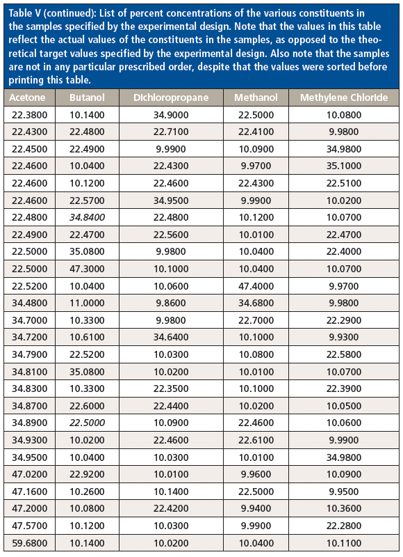
Table V (continued): List of percent concentrations of the various constituents in the samples specified by the experimental design. Note that the values in this table reflect the actual values of the constituents in the samples, as opposed to the theoretical target values specified by the experimental design. Also note that the samples are not in any particular prescribed order, despite that the values were sorted before printing this table.

On the other hand, when we are dealing with data from real mixtures, and only have some finite number of randomly selected representative mixtures, what is going on "under the hood" is not always clear. This is illustrated in the graphs presented in Figure 3, where the theoretical continua are overlaid with individual points representing samples randomly selected from the continuous values. From the way they were constructed, we know that each of the data points in Figure 3 lies on one of the lines, and therefore shares in the nonlinear nature of that line. For the n-heptane and dichloromethane, it can be seen that there is curvature in the plot of the data points, if not by themselves, then certainly by comparison, with straight lines superimposed on each of those graphs.

For the toluene, however, this is not the case. Since the sense of the curvature of some of the lines is opposite to the sense of the curvature of others of the lines, the "averaging" effect mentioned above makes the overall appearance of the graph look like there is a linear relationship between the weight fraction and volume fraction expressions of the concentrations. This is an artifact, however, one that gives the appearance of linearity when all the underlying relationships are inherently nonlinear. Thus, we've termed this relationship as being faux-linear (as in the title to this subsection). In this situation the nonlinearity cannot be detected, and the results appear to indicate only a much-exaggerated random error.

Further analysis of this data set will be considered in a subsequent column.

References

(1) H. Mark and J. Workman, Spectroscopy 25(5), 16–21 (2010).

(2) H. Mark and J. Workman, Spectroscopy 25(6), 20–25 (2010).

(3) H. Mark and J. Workman, Spectroscopy 25(10), 22–31 (2010).

(4) H. Mark and J. Workman, Spectroscopy 26(2), 26–33 (2011).

(5) H. Mark and J. Workman, Spectroscopy 26(5), 12–22 (2011).

(6) H. Mark and J. Workman, Spectroscopy 26(6), 22–28 (2011).

(7) H. Mark and J. Workman, Spectroscopy 26(10), 24–31 (2011).

(8) H. Mark and J. Workman, Spectroscopy 27(2), 22–34 (2012).

(9) H. Mark and J. Workman, Spectroscopy 27(5), 14–19 (2012).

(10) H. Mark and J. Workman, Spectroscopy 27(6), 28–35 (2012).

(11) H. Mark and J. Workman, Spectroscopy 27(10), 12–17 (2012).

(12) H. Mark and J. Workman, Spectroscopy 29(2), 24–37 (2014).

(13) H. Mark and J. Workman, Spectroscopy 29(9), 26–31 (2014).

(14) H. Mark and J. Workman, Spectroscopy 30(2), 24–33 (2015).

(15) H. Mark, R. Rubinovitz, D. Heaps, P. Gemperline, D. Dahm, and K. Dahm, Appl. Spect. 64(9), 995–1006 (2010).

(16) H. Mark, Spectroscopy25(5), 32–62 (2010).

(17) W. Windig, Chemomet. and Intell. Lab. Syst. 36, 3–16 (1997).

(18) W. Windig and D.A. Stephenson, Anal. Chem. 64, 2735–2742 (1992).

(19) G. Beranovic, Appl. Spect.71, 1039–1049 (2017).

(20) H. Mark, Eastern Analytical Symposium, Somerset, NJ, Paper #279, Nov. 18-20 (2013).

Jerome (Jerry) Workman Jr.

Jerome (Jerry) Workman Jr. serves on the Editorial Advisory Board of Spectroscopy and is the Senior Technical Editor for LCGC and Spectroscopy. He is also a Certified Core Adjunct Professor at National University in San Diego, CA and a Principal at Biotechnology Business Associates. He was formerly the Executive Vice President of Research and Engineering for Unity Scientific and Process Sensors Corporation.

Howard Mark

Howard Mark serves on the Editorial Advisory Board of Spectroscopy and runs a consulting service, Mark Electronics, in Suffern, New York. Direct correspondence to: SpectroscopyEdit@UBM.com