Multiscale Convolutional Neural Network of Raman Spectra of Human Serum for Hepatitis B Disease Diagnosis

In this study, we proposed a multiscale convolutional neural network (MsCNN) that can screen the Raman spectra of the hepatitis B (HB) serum rapidly without baseline correction. First, the Raman spectra were measured in the serums of 435 patients diagnosed with a HB virus (HBV) infection and 499 patients with non-HBV infections. The analysis showed that the Raman spectra of the serums were significantly different in the range of 400–3000 cm^-1 between HB patients and non-HB patients. Then, the MsCNN model was used to extract the non-linear features from coarse to fine in the Raman spectrum. Finally, extracted fine-grained features were placed into the fully connected layer for classification. The results demonstrated that the accuracy, sensitivity, and specificity of the MsCNN model are 97.86%, 98.94%, and 96.79%, respectively, without baseline correction. Compared to the traditional machine learning method, the model achieved the highest classification accuracy on the HB data set. Therefore, multiscale convolutional neural network provides an effective technical means for Raman spectroscopy of the HBV serum.

Hepatitis B (HB) is caused by infection with the HB virus (HBV), a kind of infectious disease dominated by liver inflammatory lesions. There are approximately two billion people infected with HBV in the world. Every year, more than one million people die of hepatic failure, cirrhosis, and hepatocellular carcinoma because of HBV infection. The incidence of HB is higher in China, and the infection rate is more than 7% (1). Therefore, we adopted the measures of “early detection, diagnosis, and treatment,” because it is the only way to improve the survival rate for HB patients.

Raman spectroscopy is a noninvasive sensitive optical analysis technique based on inelastic scattering. It also provides more molecular structure and specific fingerprint type information. It has been widely used in diagnosing the dengue fever (2), nasopharyngeal carcinoma (3), prostate cancer (4), and gastric cancer (5). Almost all types of diseases, such as cancer and infectious diseases, occur at the molecular level (6). The characteristic peak position and intensity change of Raman spectroscopy provide a basis for diagnosing diseases. Although traditional machine learning methods have been proven to be the main method for extracting feature information from Raman spectroscopy data sets in real-time, these methods require pre-processing of the data. The machine learning classification system based on Raman spectroscopy includes the following sequential preprocessing: removal of cosmic ray interference (7), smoothing, baseline correction, and using principal component analysis (PCA) to reduce the dimensionality of data (8).

The main component of the Raman spectrum background signal is caused by fluorescence, which is several orders of magnitude stronger than the actual Raman scattering (9) and resulting in inaccurate Raman data, which has a severe impact on the classification performance of machine learning. Though many scholars have achieved excellent results in this area, baseline correction remains challenging. Until now, scholars from all over the world have proposed many methods to resolve baseline correction issues, such as the polynomial baseline model (10) and simulation-based methods (11). Leon-Bejarano and others (12) proposed applying the empirical mode decomposition (EMD) method in baseline correction. Lieber and others (10) presented a modified least-squares polynomial curve fitting for fluorescence subtraction, which was shown to be effective. Zhang and others (13) proposed a variant of penalized least squares, called the adaptive iteratively re-weighted penalized least squares (AirPLS) algorithm. It iteratively adapts weights controlling the residual between the estimated baseline and the original signal.

Before we lucubrate, we should compare the application of the machine learning algorithm in Raman spectroscopy. Support vector machine (SVM) learning has been widely used in the two-class problem of Raman spectroscopy and a large part of it is related to medical applications. In this context, SVM outperforms linear discriminant analysis (LDA) and K-nearest neighbor classification (KNN) in the diagnosis of high renin hypertension (14). Although SVM excels in classification accuracy, training a nonlinear SVM is not feasible for large-scale problems involving thousands of classes. Random forest (RF) (15) is a viable alternative to high-dimensional data SVM. RF is an integrated learning method based on multidecision trees, which avoids over-delivering models to training sets. In the decade before the deep learning technique become prevalent, it was essential in the field of machine learning. However, compared with PCA-LDA and PCA-SVM (16), RF does not perform well in the classification of white blood cell subtype Raman spectra. The closest approach to convolutional neural networks is a fully connected artificial neural network (ANN). The sensitivity and specificity of ANN in Alzheimer’s disease identification is more than 95% (17). Unlike convolutional neural networks (CNN), ANN is a shallow architecture that does not have enough capacity to solve large-scale problems. Maquel and others (18) determined the primary grouping of data before conducting multi-layer artificial neural network analysis. However, Yan and others (19) used the convolutional neural network to share convolution kernels and easily process high-dimensional data and identified the sensitivity and specificity of tongue squamous cell carcinoma reaching 99.07 and 95.37%. Wang and others (20) combined serum Raman spectroscopy technology and long-short-term memory neural network (LSTM) to quickly screen HB patients with an accuracy rate of 97.32%, but the author did not consider the impact of baseline correction on the classification of machine learning model and deep learning model.

One disadvantage associated with traditional machine learning methods such as SVM, LDA, and RF is that they all require baseline corrections for Raman spectroscopy and are not easily extended to problems involving a large number of classes. Because deep learning techniques have had enormous success in computer vision, natural language processing, and bioinformatics in recent years, we proposed a network architecture for one-dimensional spectral data classification. Different from current machine learning methods, MsCNN combines pre-processing, feature extraction, and classification into a single architecture. Another important note regarding MsCNN is that it also removes the steps of baseline correction and smoothing.

Materials and Methods

Preparation of Serum Samples and Determination of Raman Spectroscopy

In this study, 435 HB patients and 499 non-HB patients from the First Affiliated Hospital of Xinjiang Medical University were included in the study group. Then, 5 mL of peripheral blood samples were collected from each subject to the blood collection tube without any anticoagulant. After the blood was fully clotting, the blood samples were centrifuged at 3000 r/min (1730 g) for 10 min to remove blood corpuscle, fibrinogen, and other components to obtain serum.

We used a laser Raman spectrometer to generate laser light at 532 nm. The spectrum was recorded in the Raman shift range of 400–3000 cm^-1, the spectral resolution was 5 cm^-1, and the recording time was 1.0 s. The LabSpec6 software package of Horiba Scientific was used to analyze the Raman spectrum data sets.

All of the above samples were from the First Affiliated Hospital of Xinjiang Medical University. With the approval of the Ethics Committee, the human serum samples were studied.

Multiscale CNN Model

In this paper, we used the modified residual network structure (21) as the building block of the multiscale convolutional neural network model. The original and our modified building blocks are shown in Figure 1. The modified building blocks are marked as Mresblock. We found that after the quick connection of the original remaining components, removing the modified linear unit and adding the Max-pool unit can improve the convergence speed during training.

FIGURE 1: (a) and (b) respectively show the structure of the original residual block and the modified residual block. For blocks with strides, the original residual block uses a convolution operation with a stride of two to align the output shape. The Mresblock uses stride operations in each block.

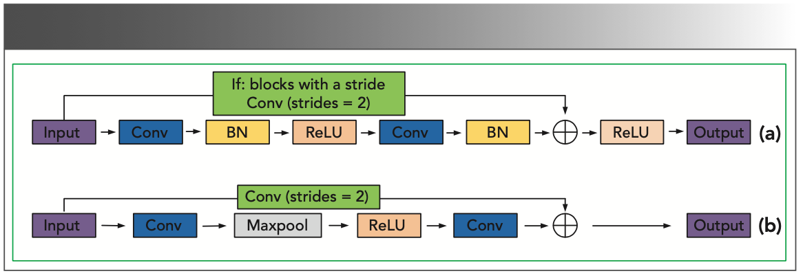
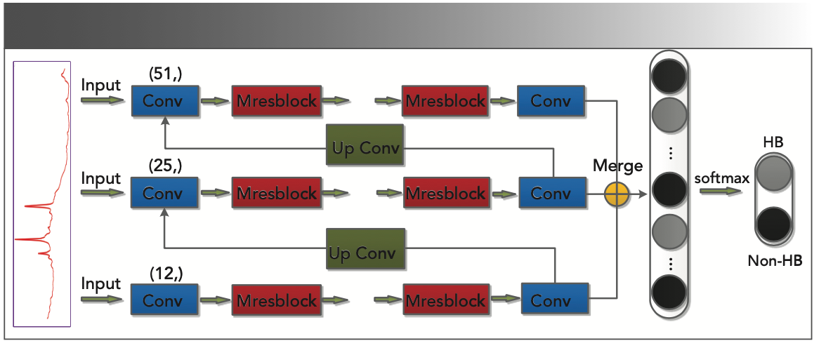
To preserve the fine-level information and simultaneously mine the coarse and intermediate information, the input and output of the network are in the form of a Gaussian pyramid. Compared with the common architecture, the residual network structure can be used to implement a deeper CNN. Because of the addition of the Max-pool unit, the size of the feature map will become half the size of the previous feature map after each Mresblock block is stacked. Therefore, the number of Mresblocks for each scale stack is different, and the number of layers stacked from top to bottom is {5, 4, 3}, and the total number of convolutions of the model is 42. At the front end of the network are three convolutional layers of different sizes (51 × 1, 25 × 1, and 12 × 1), respectively, generating 64 feature maps, and extracting spectral features of different input scales by stacking Mresblock. In addition, the information from the coarsest level output will be passed to the next stage, learning more detailed features, using up-convolution to learn the appropriate features helps to remove redundant information (22). Then, the extracted different scale features are feature-fused, and the best features learned by each scale are retained. Finally, the classification results are obtained through the fully connected layer and the classification layer. Figure 2 shows the graphical description of the network.

FIGURE 2: Multiscale convolutional neural network architecture. The input to the original spectrum is in the form of a pyramid and each scale is trained. At the time of testing, the raw spectrum size was entered.

Multiscale CNN for Raman Spectral Data Classification

The input of MsCNN in Raman spectral classification is one-dimensional, and the convolution layer is represented as follows:

Where xⁱ and yⁱ represent the input–output mapping; k is the convolution kernel, the size of the convolution kernel in Mresblock is 3 × 1; “*” is the convolution operation; and bⁱ is the offset.

We use the activation function ReLU (23), which is defined as:

Max-pooling is a further operation of spectral data, which can reduce program parameters and retain important features.

Among them, x_jⁱ and yⁱ represent the input and output of the pooling layer, and m is the largest pooling size.

The fully connected layer follows the convolutional layer, and finally, the number of outputs from the Softmax layer is equal to the number of classes considered. In the fully connected layer, we use ReLU as the activation function. Softmax is a compression function. It can compress a K-dimensional vector z containing any real number into another K-dimensional real vector so that the range of each element is between [0, 1], and the sum of all elements is 1.

Loss Function

The coarse-to-fine approach desires that every intermediate output becomes the feature map of the corresponding scale. Therefore, the intermediate output of our training network should form the form of a Gaussian pyramid. The MSE standard applies to every level of the pyramid. The loss function is defined as follows:

Here n is the batch size, y_n is the training data tag, and p_n is the result of the output layer.

The training of the MsCNN was performed using the Adam algorithm, which is a variant of stochastic gradient descent, for 100 epochs with learning rate equal to 1e-3, β₁ = 0.9, β₂ = 0.999, and ε = 1e-8. The layers were initialized from a Gaussian distribution with a zero mean and variance equal to 0.05. The training was performed on a single Nvidia RTX-2070 GPU.

Evaluation Protocol

We tested the MsCNN model on the Raman spectroscopy data set of HB serum. First, we conduct a series of ablation experiments on the original spectral data. Then compared with many machine learning algorithms in the past for spectral recognition. The contrast experiment was divided into two groups. The first group was the pre-processed spectral data, and the second group was the original spectral data. During the preprocessing of data, Savitzky-Golay (with nine points and 5th order polynomial fitting) (24) method was used to smoothen the spectral data. Then adaptive iterative reweighted penalty least squares (AirPLS) algorithm was used to correct the baseline (13). We use principal component analysis to extract key features of the data, retaining 99.99% of the total variance (51 dimensions). During model training, five-fold cross-validation is used to evaluate the model.

The machine learning algorithms involved in the comparison included KNN, RF, LDA, ANN, SVM, CNN, and ResNet. The evaluation indicators of the above algorithms included accuracy, sensitivity, and specificity. Accuracy takes into account both positive and negative probabilities of the model, which is of high global significance. Sensitivity is also called a valid positive rate—the higher sensitivity, the lower likelihood of missed diagnosis. Specificity is also called exact negative rate—the higher specificity, the higher probability of confirmed diagnosis. The proposed MsCNN was applied using Keras (25) and Tensorflow (26). All other machine learning methods are implemented using Scikit-learn (27).

Results and Analysis

Raman Spectroscopy

Figure 3 shows the mean spectra and difference spectrum after baseline correction of serum from HBV patients’ samples and non-HBV patients’ samples in the range of 400 cm^-1 to 3000 cm^-1. It demonstrates that the mean spectra of HBV and non-HBV samples are almost identical in structure, with only minor changes in the intensity of some Raman bands that can’t be detected by naked eyes. Direct visual interpretation can very likely result in misdiagnosis. There is an urgent need for a method to distinguish the lesion sample from the standard sample accurately.

FIGURE 3: Normalized average spectra and difference spectrum (black) of samples from hepatitis B patients (red) and non-hepatitis B patients (green).

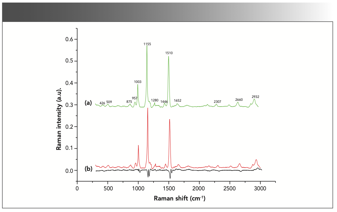
Raman peaks at 426, 509, 875, 957, 1003, 1155, 1280, 1446, 1510, 1652, 2307, 2660, and 2932 cm^-1 can be observed in both groups, with the most energetic intensities at 1003, 1155, 1510, and 2932 cm^-1. These intensity differences in the Raman spectra can be viewed more clearly at the bottom of Figure 3 that means, there is excellent potential for identifying HBV patients and healthy person using Raman spectra of serum.

Multiscale Ablation Experiments

We conducted a series of ablation experiments on the original data set. These data retained 99.99% of the total variance (51 dimensions) through principal component analysis. The first scale is 51 dimensions, and the remaining scale is 1/2 of the previous scale. Specific experimental results are shown in Table I.

As can be seen from Table I, when using two different scales (line 2 of Table I) to classify the primitive data, the performance is better than the model using the same scale, and its accuracy, sensitivity, and specificity are 96.11%, 95.37%, and 95.79%, respectively. In addition, in the experimental comparison of different scales, the overall results of the MsCNN model using three scales are superior to other scales. Therefore, we ended up using three different scales of MsCNN as the model in this paper.

Baseline Correction Spectral Classification

We evaluated our MsCNN method on a HB data set. These spectra had been baseline corrected, and cosmic rays had been removed too. Then, we followed the pre-processing techniques and evaluation criteria described in Section 2.5. The experimental results are shown in Table II.

It can be seen from Table II that the KNN model has the worst classification effect, with an accuracy rate of only 78.07%. The ANN model has the highest sensitivity (98.00%), but as the number of neurons increased during the training process, the slower the training speed and the lower the efficiency. ResNet uses its deeper network structure to mine more information, and the accuracy is up to 96.31%, which is 1.52% higher than the ordinary CNN model. As one of the most commonly used machine learning classification models, SVM has an accuracy rate of 94.25%, which is 2.27% and 6.55% higher than the accuracy of the RF and LDA models, respectively. In addition, the use of deep learning methods to identify baseline-corrected spectra is better than previous machine learning methods. The accuracy of the MsCNN model is the highest among all models (96.79%), which demonstrates the effectiveness of the improved Mresblock module in this article. And it proves that the deep learning method has great potential in extracting Raman spectral feature information at the same time.

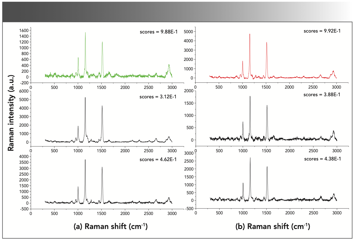
To understand the MsCNN model better, we also studied the model prediction, especially those were not consistent with the correct labels. Figure 4 shows the spectra of the HB patient (shown in red) and the non-HB patient (shown in green) that have the most accurate model predictions. It also shows the spectra with wrong predictions. We found that the processed data has a highly similar spectral structure. By observing the two correctly classified spectra, we saw that the Raman peak of HB patient is much higher in value than non-HB patient. Performing similarity analysis from the peak, MsCNN model may classify HB patient in group B as non-HB patient. Because of the predicted spectrum, B has a high peak similarity to the correctly classified spectrum in A. These plots demonstrate that the MsCNN can match the peaks characteristic of a particular species even when the prediction did not agree with the correct label.

FIGURE 4: Examples of successful and unsuccessful classification. In the figure, the green (a) and red (b) spectra in the first row represent the predicted spectra of non-HB patients and HB patients, respectively. The second and third rows are the corresponding category spectra that were incorrectly predicted. The prediction score is also shown in each figure, reflecting the confidence of the prediction.

Classification of Primitive Spectra

The results show that MsCNN is able to achieve significantly better accuracy compared to other conventional machine learning methods on the baseline corrected spectra. In this section, we explored the performance of MsCNN on data without baseline processing. Before the experiment, except for RF, only 99.99% of the total variance of PCA had been used to reduce the data dimension, because we found that PCA reduces the performance of RF. The experimental results are shown in Table III.

As can be seen from Table III, the deep learning method has a great advantage in processing the original high-dimensional data. Analyzing and contrasting the results in the “Multiscale Ablation Experiments” section and the experimental results in this section, we can observe that baseline correction significantly improves the performance of all the conventional methods by 4–5%. That is because the baseline correction removes the effects of signal compression and other noise from natural bioluminescent vectors. On the other hand, the performance of MsCNN drops by approximately 0.5–2% when combined with baseline correction methods. This result may indicate that MsCNN can learn the technique of dealing with baseline interference more effectively than the baseline correction method and retain more identification information. The use of coarse-to-fine methods for training in multi-scale spaces is better suited for Raman spectroscopy.

Discussion

Here, we reported the application of the Raman spectrum of serum combined with multiscale CNN methods for HB patients screening. Through the analysis of the mean spectrum of HBV infection and non-HBV infection groups, we found that peak changes in Raman spectra of serum may be related to many vibrational modes of various biomolecules such as lipids, proteins, and nucleic acid molecules. Table IV lists tentative assignments for the dominant spectral bands according to the previous literature (28).

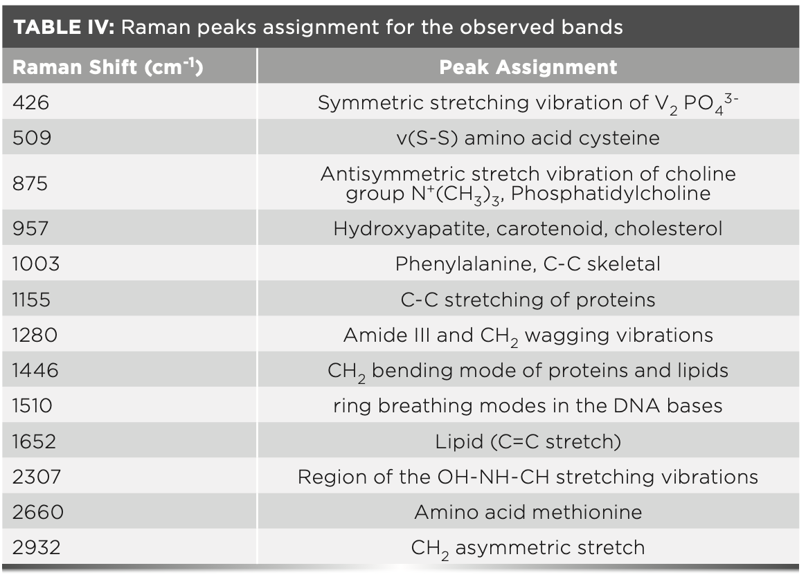
For some peaks, such as 509, 957, 1003, 1155, 1510, and 2660 cm^-1, the intensities of the pathological samples are higher than the standard samples. An increase in the intensity of Raman peak at 509 cm^-1 is because of cysteine. Cysteine is a sulfur-containing amino acid. If its value is too high, it may cause abnormal liver function, resulting in severe functional disorders such as hepatocyte synthesis and metabolism. When liver cell damage is mild, the healthy metabolic function of the liver cell will not cause the change of cysteine level (29). Raman peak at 2660 cm^-1 is assigned for amino acid methionine, in the literature (30), the researchers found that plasma fragrant amino acids and methionine levels were significantly elevated in patients with liver disease. Raman peak at 957 cm^-1 is because of cholesterol. High cholesterol content will further damage the liver of HB patients, increases the burden on the liver, causes fat metabolism disorder, and affects the digestive function of HB patients, this is consistent with the conclusion that the serum cholesterol levels of patients with coronary heart disease and liver disease are relatively elevated in the literature (31). Raman peak at 1510 cm^-1 is mainly because of the ring breathing mode of DNA bases (28). The Raman peak of Phenylalanine in serum albumin is 1003 cm^-1. An elevated level of Phenylalanine is most likely because of dysfunction of the liver in HBV infected patients (32,33). Increases in these intensities of Raman peaks indicate the augment of albumin concentration in the blood of HBV infected person. The peak at 1155 cm^-1 belongs to the vibration of carotenoids (34). It can be seen from Figure 3 that the carotenoid content in the blood of patients with HB is much higher than that in non-HB patients. Carotenoids are an antioxidant that plays an important role in protecting cells and organisms from free radicals (ROS) and reactive nitrogen (RNS) free radicals. Li and others (35) showed that the application of antioxidants is a reasonable treatment strategy for the prevention and treatment of liver diseases. Therefore, the content of carotenoids in patients with HB is much higher than that in patients with non-HB. It may be to relieve liver cirrhosis and even liver cancer in patients with HB.

In contrast to the above, Raman bands 875, 1280, 1446, 1652, and 2932 cm^-1, decreased intensities, have been observed for the diseased sample. A peak at 875 cm^-1 is because of antisymmetric stretch vibration of choline group N⁺(CH₃)₃. Phosphatidylcholine has the effect of repairing an alcoholic liver injury, fatty liver, and preventing cirrhosis (36). Non-HBV patients have a slightly higher peak at 875 cm^-1 than HBV patients, probably because phosphatidylcholine metabolism is relatively active in non-HBV (37). Likewise, the intensity of Raman peak assigned to lipids owning to the C=C stretch (28) also decreased at 1652 cm^-1. Raman peaks at 1280 cm^-1 and 2933 cm^-1 are because of C-H stretching and assigned for amide III. A decrease in the peak intensity at 1280 and 2933 cm^-1 shows decrease concentration of β-sheet in HBV infected patients, which is in agreement with the existing literature that reported that a decrease in beta structure compared to the helical structure in the amide III region is an indication of interferon secretion by lymphocytes as an immune response against HBV infections (38).

Conclusion

In this study, we proposed a Raman spectral classification method, which not only has an excellent performance but also avoids baseline preprocessing, for MsCNN. Our approach has been validated on the HB data set and has proven to be largely superior to other traditional machine learning methods. Although we focused our study on Raman data of HB serum, we believe the technique is also applicable to Raman spectroscopy of serum for other diseases. We speculate that Raman spectroscopy of serum has similarities, and fine-tuning our network can make it very practical to classify new problems. This process is called migration learning, which has been widely used in image recognition and natural language processing.

Acknowledgments

This work was supported by the National Natural Science Foundation of China (NSFC) (No. 61765014); Reserve Talents Project of National High-Level Personnel of Special Support Program (QN2016YX0324); Urumqi Science and Technology Project (No. P161310002 and Y161010025); and Reserve Talents Project of National High-level Personnel of Special Support Program (Xinjiang [2014]22).

Disclosures

The authors declare no conflicts of interest.

References

(1) S. Velkov, J.J. Ott, U. Protzer, and T. Michler, Zeitschrift für Gastroenterologie 57, P5–P50 (2019). doi: 10.1055/s-0038-1677297.

(2) T. Mahmood, H. Nawaz, A. Ditta, M.I. Majeed, M.A. Hanif, N. Rashid, et al., Spectrochim. Acta. A. 200, 136 (2018). doi:10.1016/j.saa.2018.04.018.

(3) S. Feng, R. Chen, J. Lin, J. Pan, G. Chen, Y. Li, et al., Biosens. Bioelectron. 25, 2414–2419 (2010). doi:10.1016/j.bios.2010.03.033.

(4) S. Li, Y. Zhang, J. Xu, L. Li, Q. Zeng, L. Lin, et al., Appl. Phys. Lett. 105, 91104 (2014). doi: 10.1063/1.4892667.

(5) L. Guo, Y. Li, F. Huang, et al., J. Innov. Opt. Health Sci. 12(02), 1950003 (2019). doi: 10.1142/s1793545819500032.

(6) S. Khan, R. Ullah, A. Khan, R. Ashraf, H. Ali, M. Bilal, et al., Photodiagn. Photodyn. 23, S254044298 (2018). doi:10.1016/j.pdpdt.2018.05.010.

(7) Z. Bai, H. Zhang, H. Yuan, J.L. Carlin, G. Li, Y. Lei, et al., Publ. Astron. Soc. Pac. 129, 24004 (2016).

(8) P.B. Garcia-Allende, O.M. Conde, J. Mirapeix, A.M. Cubillas, and J.M. Lopez-Higuera, IEEE. Sens. J. 8, 1310–1316 (2008).

(9) S. Chen, L. Kong, W. Xu, X. Cui, and Q. Liu, IEEE. Access. 6, 67709–67717 (2018). doi: 10.1109/ACCESS.2018.2879160.

(10) C.A. Lieber and A. Mahadevan-Jansen, Appl. Spectrosc. 57, 1363–1367 (2003). doi: 10.1366/000370203322554518.

(11) M.A. Kneen and H.J. Annegarn, Nucl. Instrum. Meth. B. 109–110, 209–213 (1996). doi: 10.1016/0168-583x(95)00908-6.

(12) M. Leon-Bejarano, G. Dorantes-Mendez, M. Ramirez-Elias, M.O. Mendez, A. Alba, I. Rodriguez-Leyva, et al., Conf. Proc. IEEE. Eng. Med. Biol. Soc. 3610–3613 (2016). doi: 10.1109/EMBC.2016.7591509.

(13) Z. Zhi-Min, C. Shan, and L. Yi-Zeng, Analyst 135, 1138 (2010). doi: 10.1039/b922045c.

(14) X. Zheng, G. Lv, Y. Zhang, X. Lv, Z. Gao, J. Tang, et al., Spectrochim. Acta. A. 215, 244–248 (2019). doi:10.1016/j.saa.2019.02.063.

(15) I. Barandiaran, IEEE. Trans. Pattern. Anal. Mach. Intell. 20, 1–22 (1998). doi: 10.1109/34.709601.

(16) A. Maguire, I. Vega-Carrascal, J. Bryant, L. White, O. Howe, F.M. Lyng, et al., Analyst 140, 2473–2481 (2015). doi:10.1039/C4AN01887G.

(17) E. Ryzhikova, O. Kazakov, L. Halamkova, D. Celmins, P. Malone, E. Molho, et al., J. Biophotonics 8, 584–596 (2015). doi:10.1002/jbio.201400060.

(18) K. Maquelin, C. Kirschner, L. Choo-Smith, N.A. Ngo-Thi, T. Van Vreeswijk, M. Stämmler, et al., J. Clin. Microbiol. 41, 324–329 (2003). doi: 10.1128/JCM.41.1.324-329.2003.

(19) H. Yan, M. Yu, J. Xia, et al., Vib. Spectrosc. 2019, 102938. doi:10.1016/j.vibspec.2019.102938.

(20) X. Wang, S. Tian, and L. Yu, et al., Lasers in Med. Sci. 35(8), 1791–1799 (2020).

(21) K. He, X. Zhang, S. Ren, et al., “Deep Residual Learning for Image Recognition,” paper presented at the 2016 IEEE Conference on Computer Vision and Pattern Recognition (CVPR), pp. 770–778 (2015). doi: 10.1109/CVPR.2016.90.

(22) J. Long, E. Shelhamer, and T. Darrell, IEEE. T. Pattern. Anal. 9(4), 640–651 (2014). doi:10.1109/TPAMI.2016.2572683.

(23) P. Sharma and A. Singh A., “Era of deep neural networks: A review,” paper presented at the International Conference on Computing, Communication and Networking Technologies (ICCCNT), pp. 1–5 (2017). doi: 10.1109/ICCCNT.2017.8203938.

(24) A. Savitzky and M.J. Golay, Anal. Chem. 36, 1627–1639 (1964). doi:10.1021/ac60214a047.

(25) T.B. Arnold, J. Open Source Software 2, 296 (2017). doi:10.21105/joss.00296.

(26) L. Rampasek and A. Goldenberg, Cell Syst. 2, 12–14 (2016). doi:10.1016/j.cels.2016.01.009.

(27) W. Wang, J. Xi and D. Zhao, IEEE Transactions on Vehicular Technology 67(5), 3887–3899 (2018). doi:10.1109/TVT.2018.2793889.

(28) Z. Movasaghi, S. Rehman, and I.U. Rehman, Appl. Spectrosc. Rev. 42, 493–541 (2007). doi:10.1080/05704928.2014.923902.

(29) B.L. Urquhart, D.J. Freeman, and J.D. Spence, et al., Am. J. Kidney. Dis. 49(1), 109–117 (2007). doi: 10.1053/j.ajkd.2006.10.002.

(30) C. Loguercio, F.D. Blanco, G.V. De, et al., Alcohol. Clin. Exp. Res. 23(11), 1780–1784 (2010). doi: 10.1111/j.1530-0277.1999. tb04073.x.

(31) N.P. Odushko and N.F. Muliar, Kardiologiia 24(10), 90 (1984).

(32) M.J. Baker, S.R. Hussain, L. Lovergne L, et al., Chem. Soc. Rev. 45, 1803–1818 (2016). doi: 10.1039/C5CS00585J.

(33) A. Rygula, K. Majzner, K.M. Marzec, et al., J. Raman. Spectrosc. 44(8), 1061–1076 (2013). doi: 10.1002/jrs.4335.

(34) N. Tschirner, M. Schenderlein, K. Brose, et al., Phys. Chem. Chem. Phys. 11(48), 11471 (2009). doi: 10.1039/B917341B.

(35) L. Sha, T. Hor-Yue, and W. Ning, et al., Int. J. Mol. Sci. 16(11), 26087–26124 (2015). doi:10.3390/ijms161125942.

(36) G. Buzzelli, S. Moscarella, A. Giusti, et al., Int. J. Clin. Pharm-Net. 31(9), 456 (1993).

(37) W.J. Schneider and D.E. Vance, Cent. Eur. J. Biol. 85(1), 181–187 (2010). doi: 10.1111/j.1432-1033.1978.tb12226.x.

(38) J.D. Gelder, K.D. Gussem, and P. Vandenabeele, et al., J. Raman. Spectrosc. 38(9), 1133–1147 (2007). doi: 10.1002/jrs.1734.

Junlong Cheng and Long Yu are with the College of Information Science and Engineering at Xinjiang University, in Urumqi, China. Shengwei Tian and Xiaoyi Lv are with the College of Software Engineering at Xin Jiang University, in Urumqi, China. Zhaoxia Zhang is with the First Affiliated Hospital of Xinjiang Medical University, at Urumqi, China. Direct correspondence to: tianshengwei@163.com ●