Outliers, Part II: Pitfalls in Detecting Outliers
Spectroscopy
How can you detect the presence of an outlier when it is mixed with multiple other, similar, samples?
This column is part II of our series dealing with the question of outliers. Here we consider some of the methods that have been devised to detect the presence of an outlier when it is mixed in with multiple other, similar, samples.
Whether we did it well or badly, in the previous column (1) we discussed the concept of what an outlier is. The next point to consider is how to detect an outlier, in the face of the inherent fuzziness of the concept. This means that we will not always be correct in the assessment of any particular suspect datum, but here we will look at various situations and seek universal methods (which may or may not exist).
A common way to detect outliers is to plot the data and look for readings that are "far away" (in some sense, as judged by the viewer's eye) from the behavior of the rest of the data in the given set under consideration. In particular, if the data being examined are the result of a multivariate calibration and the computer is plotting the predicted values from the calibration model versus the reference laboratory results (or even better, the residuals from the calibration versus the reference laboratory results), we expect the plot to follow what is called the "45° line" (or a flat line, if the residuals are being plotted), with the random error causing the individual data points being normally distributed (that is, conforming to the Gaussian distribution; all occurrences of "normal" in this column have that meaning) around that line. This isn't a bad way to examine calibration results, as long as you're aware of the traps and pitfalls that abound.
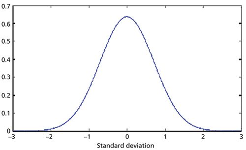
Figure 1: The theoretical normal distribution.
For example, as a statistical problem, we must be aware that we have to deal in probabilities. For instance, everyone knows that for a normal distribution, 95% of the readings should be within two standard deviations of the center of the distribution, and 99% of readings should be within three standard deviations. Anything beyond those limits is considered the "forbidden zone," in which no samples should be found. So the conclusion jumped to is that a reading beyond three standard deviations is unlikely to occur, and therefore any reading beyond three standard deviations must be an outlier. Figure 1 shows the normal distribution, as a function of the standard deviation, and we can see how, beyond ±2 standard deviations, the probability of obtaining a value in that region becomes very small. What is missing in that line of reasoning is the fact that the probability levels given for various values of the normal distribution correspond to the probability of getting that value when selecting a single random sample from the distribution. When more than one sample is taken into consideration, the probability of one or more samples falling in the specified region increases since any sample can fall into the "forbidden zone" independently of the other samples. We have discussed this effect previously (see chapter 1 in reference 2).
In this situation, the actual probability of any of a multiplicity of samples falling into the forbidden zone is given by the following equation:

where Pi is the probability of any individual reading being within the allowed limits (generally 0.95), P is the actual probability that any reading from the set is outside the limit, and n is the number of readings (or data points).
For a single sample, then, if a single (random) sample has a probability of 0.95 of being within the "normal" range then the probability of being outside that range (that is, in the "forbidden" region) is 0.05. This probability is considered small enough to declare that a sample found in the forbidden region must have something wrong with it.
As a numerical example, if we have 20 readings from a set of (presumably normally distributed) errors and we are concerned about the probability of a reading being beyond the ±2 standard deviation limit, then we can substitute the numbers into equation 1 to get

That is, almost two-thirds of the time, at least one reading will fall in the "forbidden" zone beyond two standard deviations, because of the random variability of the data alone, with no unusual special circumstance affecting it. This is hardly proof of something unusual about that reading.
For 100 readings the probability becomes 0.9941-almost a certainty that at least one sample will be beyond the specified limit. Thus, using this criterion to identify outliers will ensure that perfectly acceptable readings will be falsely identified as outliers.
Another way to look at the situation is that a probability of 5% means that one sample in 20 will fall in the region beyond ±2 standard deviations. If we have 100 samples, therefore, roughly five of them should be in that "forbidden" region of the distribution; if there are no samples there, something is wrong-fully five samples should be in the "forbidden" zone. To have none there is the "rare event."
Can anything be done? Answer: yes. We can reset the probability test levels to correspond to a true 0.95 probability for a set of multiple samples by solving equation 1 for Pi:

In words, equation 2 tells us that for n readings, we have to perform our statistical tests at a probability level that is the nth root of the desired probability. Thus, if we have 100 readings (residuals, say) and we want to test at a true value of 95% probability, then we must perform the test against the number of standard deviations corresponding to 0.95(1/100) = 0.9995, which corresponds roughly to 3.5 standard deviations. This means that if your sample set contains 100 samples worth of data and you want to use this type of test for detecting outliers, or any test that is supposed to be based on single readings, you have to set the threshold for the test at 3.5 standard deviations to get a true significance level of 0.95. Since the probability level to use depends on the number of samples, this test would quickly become unwieldy for routine use.
Another pitfall is encountered when we consider the actual distribution of data randomly sampled from a normal distribution. Figure 1 presents a very pretty display of the normal distribution, representing the mathematically ideal situation. Reality, we're afraid, isn't nearly so neat. In Figure 2 we used the MATLAB "randn" function to create datasets of various sizes, all taken randomly from the normal distribution, then plotted the histogram of the actual distributions for each such (relatively small) sample taken. These randomly selected, normally distributed numbers are representative of the behavior of errors in a calibration situation. For each sample size, the selection and histograms were repeated five times, to illustrate the variability caused by the randomness. We plotted the distribution histograms as line graphs to avoid the plots becoming too busy. The numbers of samples used (30 to 500) were chosen to more-or-less correspond to the range of number of samples typically used for near-infrared (NIR) calibrations.
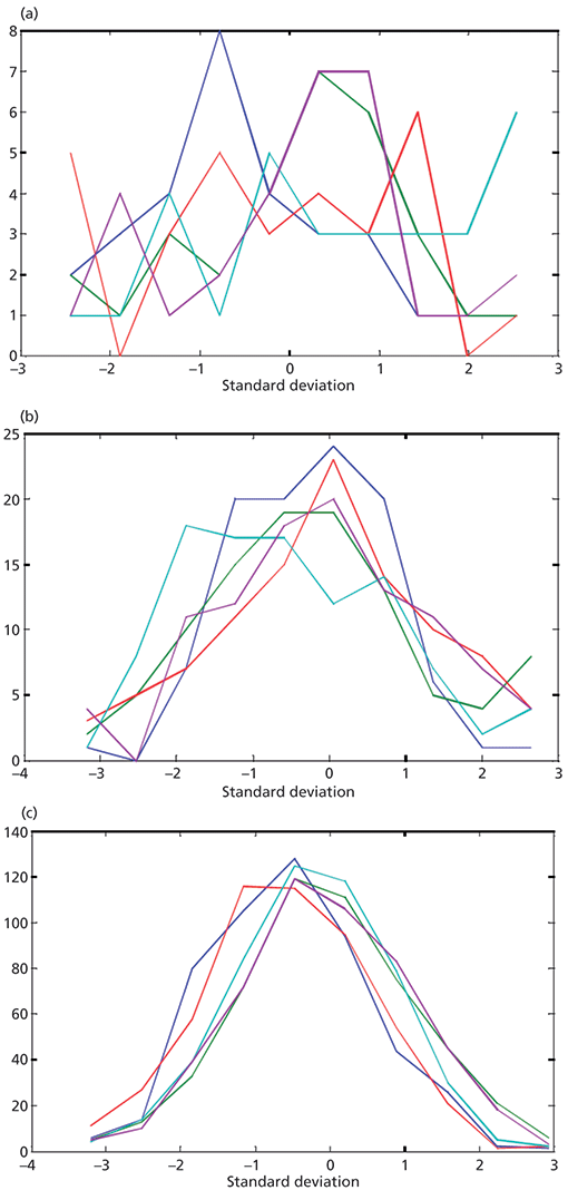
Figure 2: Actual distributions (histograms) of samples of various numbers of readings taken from the normal distribution, showing the actual distributions of values achieved, for each case. For each part of this figure the random sampling was repeated five times, to allow the variability of the data to be seen. The plots show distributions of (a) 30, (b) 100, and (c) 500 random readings.
We see that when only 30 samples are used it's almost impossible to tell that the underlying distribution is normal (rather than, say, uniform), much less set meaningful confidence limits for outlier detection. For 100 samples we can tell that the probability maximum is somewhere around the middle of the set of data, but it still doesn't look like anything close to normal. At 500 samples we see that some tails are starting to be noticeable, but just barely.
As far as detecting outliers goes, however, the numbers of samples used for these demonstrations are sufficient to show the variability of the distributions and their likely effects on setting thresholds, but these histograms, using only 10 intervals for the histogram, are insufficient for us to examine what is happening at the extremes of the range, where the information that is interesting to us for detecting outliers, will be found. We will now, therefore, examine examples of this same distribution using different numbers of bins in the histogram. The histograms in Figure 2 all used 10 bins to generate the histogram. In Figure 3 we use varying numbers of bins to examine the effects of the binning on the distribution of 500 samples from a randomly sampled normal distribution. In Figure 3 we also use bar graphs to plot the histograms, giving us the more familiar presentation of the histogram; for this reason we only present the histogram from a single set of this simulated data.
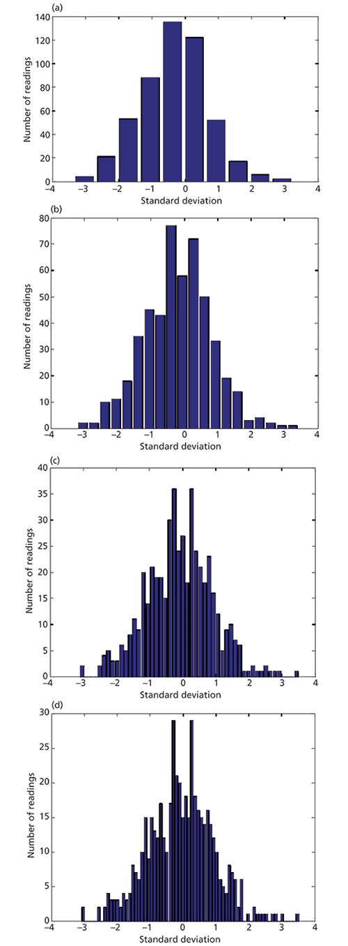
Figure 3: Histograms for 500 normally distributed numbers (representing errors in a calibration) in histograms using (a) 10, (b) 20, (c) 50, and (d) 70 bins. These histograms were all generated from the same set of random numbers.
In Figure 3, we see that binning the data into 10, and even 20 bins, pretty well reproduces what we saw in Figure 2: The distribution appears normal to the eye (albeit slightly asymmetric, to be sure). With 50 or more bins, however, we can see the erratic nature of the distribution at the two extremes of the range, with relatively large sets of empty bins sometimes appearing between bins containing samples.
So, how does all this affect our methods of analyzing calibration plots? Figure 4 shows a simulated calibration plot using synthetic data representing 100 samples with characteristics similar to what are found in many calibration datasets. Both the x- and y-data were based on a uniform distribution of samples with a range going from 10 to 30; this is represented by the solid line. Random normally distributed numbers representing calibration errors with a standard deviation or 2 were then added to the y-data, and the individual data points were plotted as blue circles.
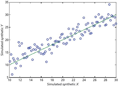
Figure 4: A simulated calibration plot showing possible outliers. See text for discussion.
Several of the plotted points appear to be suspect, based on the visual observations of the plot in Figure 4. These questionable data points include the point at x = 28.8, y = 33.9 and the cluster of three points around x = 12.0, y = 18.0, as well as a couple of data points with highly negative errors. An overeager (and probably rushed) data analyst would summarily reject those data points, deleting them from the data set.
Are these points outliers? In this case we know for a fact that they are not, since we know that these "error" terms are all legitimate parts of the normal distribution that the errors presumably comprise. The purpose of this exercise is to caution the reader against too-freely identifying and deleting marginal or suspect samples as outliers. This sort of excessive outlier deletion is one of the more likely causes of the large discrepancies seen between calibration performance and validation results. The elimination of samples from a calibration set simply because they have what appears to be large errors will ipso facto make the calibration results appear to be better than they actually are. Then, when more realistic validation values are obtained, they seem to be the source of the discrepancies seen between the two types of calibration performance, when the discrepancy is actually because of the too-small calibration error estimate created by the elimination of the larger-value errors despite their being completely legitimate.
The first part of this column, up to this point, has essentially been a warning against overzealous application of simplistic considerations, creating the danger of making what statisticians call the type 2 error: falsely identifying outliers when none exist. So then, how can we detect an outlier? Books such as the one we referenced previously (3) provide several approaches to solving this problem. Not surprisingly, they use methods other than simply counting standard deviations from the mean. Barnett and colleagues (3) also make it clear that the existence of an outlier also depends very much on the distribution of the data that the suspected outlier is supposed to fit. Our examples in Figures 1–3 are predicated on the reference distribution being the normal distribution.
In general, however, not all data are normally distributed, and any tests applied to non-normal data must either be suitably chosen to match the distribution or at least have their critical values adjusted to take into account the actual data distribution. For our examples here, however, we will consider the normal distribution to be our reference distribution. This is in keeping with our expectation in writing this column that the majority of our readership is interested in the application of the concepts we discuss to quantitative spectroscopic analysis. One of the fundamental assumptions behind the common algorithms used for that type of analysis is that the errors in the reference values are normally distributed. For other applications, of course, caveat emptor: You must properly deal with the nature of the data you collect.
Much of what we discuss here will be based on the text at hand (3). As we might expect from our recent discussions of the history of statistics (4), the early mathematicians developing the foundations of statistics were also active in these related fields of data analysis. Hence some of the same familiar names appear such as Bernoulli, Legendre, Bessel, as well as many less-familiar names such as Stone, Boscovich, Goodwin, and Chauvenet. For the most part, informal, ad hoc procedures for examining the data were recommended, much as is done today; this approach was popular until as recently as WWI. Barnett and colleagues (3) also discuss some of these early, and simplistic approaches to identifying outliers. Problems abound, and are often both subtle and disastrous. For example, Barnett and colleagues cite one of the earliest attempts to develop an objective outlier test (5) based directly on probability theory, which turned out to be very effective in identifying outliers. However, the test under consideration had the unfortunate side effect of also rejecting as many as 40% of the valid observations.
Sometimes a test having those characteristics may even be satisfactory. While we wouldn't expect this to be common, tests with asymmetric characteristics like this may sometimes be useful, depending on extraneous conditions. The test cited by Pierce, for example, could be useful if all of several conditions apply: It is critical to ensure that all outliers are removed from the data to be analyzed, there is enough data, and the data contain enough redundancy, that the loss of a few (or even several) samples' worth of data will not affect the results of the analysis. Barnett also discusses, at length, various considerations that may affect the outlier detection algorithms that might be used. Some of these considerations include the purpose for which the data will be used (as we discussed just above), the underlying distribution (or expected distribution) of the data (or of the errors, as appropriate), multiple outliers, multivariate data, and the expected action to be taken upon identifying an outlier, and others. We will not discuss these at length here, although we may address some of them briefly in passing.
Most informal, ad hoc, statistical tests for outliers, such as the one described in Figure 4, are dependent on setting a threshold for some calculated statistic to which values for that statistic for each sample are compared, and declaring an outlier when the sample's value for the statistic exceeds the threshold. By their nature, these tests are tests of the extreme samples. This type of test is basically a specialized form of hypothesis test, as described previously. Important features of outlier tests of this form include the probability of failing to detect an outlier when one is present, the probability of falsely detecting an outlier when none is present, and the immunity of the test to changes in scale of the data. Furthermore, to be considered a legitimate statistical test, the user must be able to specify the probability level at which the outlier is declared, as well as the probability for a legitimate sample to be falsely declared an outlier. Another key point that the user of any of these tests must keep in mind is whether the calculation of the reference value is to include the suspect datum. Clearly, the data point in question, being an extreme value of the data set, will have the maximum effect on the value of the threshold comparison value, compared to all the other data, so whether it is included or excluded from the calculations becomes a very important consideration.
Since we are concerned with the extreme samples in a set of data, we must keep in mind the truism that any finite data set has to have at least two extreme values. Moreover, we had previously uncovered possible pitfalls to this kind of test, in that those extreme samples are not necessarily outliers just by virtue of their characteristic of being extreme. Over the years, however, statisticians have developed ways of producing tests of the extreme samples that avoid that pitfall. Here we discuss some of them. As a reference plot for visual comparison we created a new plot as shown in Figure 5, where we have recreated the distribution of Figure 3c and artificially added an extra data point to represent an outlier. This is representative of the various tests that are proposed.
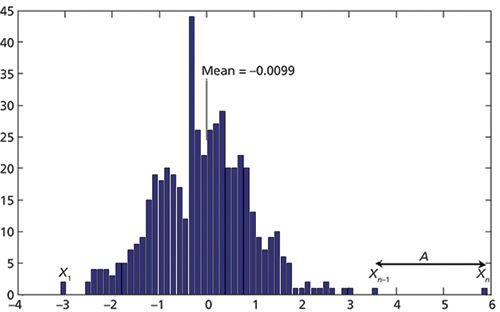
Figure 5: Histograms for 500 normally distributed numbers (representing errors in a calibration) in a histogram containing 500 data points, plus one simulated outlier.
The tests are based on the concept that there are n data points, numbered 1 to n in order. As shown in Figure 5, the first data point is labeled X1 while the last data point is labeled Xn, and the next-to-last data point is Xn-1. Then several possible alternate ways of comparing the last data point, which is presumably the suspected outlier, are proposed. As seen in Figure 5, we have labeled the difference between the most extreme reading and the second-most extreme, to emphasize that many of the tests are predicated on the comparison of the distance of the most extreme sample from other readings, rather than the distance from the center of the data, as we are usually concerned with.
Barnett and colleagues (3) present some of the simpler outlier tests that have been developed over the years, and point us to sources of corresponding threshold values for the statistics calculated by the various tests (T represents the test statistic that will be used for comparison with a threshold [critical value]).
1. T = (Xn– Xn-1)/(Xn– X2) (6). This test compares the distance of the suspected outlier from the next-highest value, to the range of the sample data. Note that the first sample is not included in the range to avoid the possibility that it is also an outlier, which would then give an incorrect threshold test value.
2. T = (Xn– Xn-1)/σ (7). This test is similar to test 1 except that the denominator contains the population standard deviation (which must therefore be known) instead of the sample range.
3. T = (Xn– Xn-1)/σ (8). Another similar test, but using the full range from the outlier in the numerator, and replacing the population standard deviation with the sample standard deviation. This test is subject to having the requirement that X1 is not an outlier itself.
4. T = (X(with macron)– Xn-1)/S (9). Testing for a lower outlier using the sample mean.

this is a more exotic formula, for testing two suspected outliers simultaneously (9).
Dixon's test functions for rejection of outliers, along with a table of critical values, has been nicely presented in an ASTM practice (10) (see Annex A1). These are a set of equations similar to equation 1 above that can be used to test large sets of data for multiple outliers.
Barnett (3) also points to some formulas using higher-order measures (skew and kurtosis) of the data, for the purpose of testing for outliers. Variations of these formulas, to avoid distortions from other outliers in the data set or some of the problems listed earlier, are obvious, although the adjustments needed for the threshold values may not be.
The above-listed outlier tests are all intended to be used for situations where the underlying distribution of values for nondiscordant readings is normal (Gaussian).
Barnett (3) also lists another extensive set of tests for discordancy from a normal distribution, for a variety of conditions. That book also presents an extensive set of tests for situations where the underlying distribution is other than normal. We present some of those here also, for reference.
For values that are gamma-distributed or exponentially distributed: Barnett provides 16 different tests suitable for various conditions. As with other tests, here we only include one of each type of test that is discussed:
The test statistic for a single upper outlier of an exponential sample is

For values that are normally distributed, Barnett lists 30 different tests, some of which duplicate the ones listed above, so we forbear repeating them.
For values that are log-normally distributed, take the logarithms of the data and apply a suitable test for data that is normally distributed.
For values that are uniformly distributed, one test uses the following test statistic:

Barnett also presents tests for situations where the underlying data distribution is Poisson, binomial, truncated exponential, Pareto, Weibull, and other unusual and exotic distributions, but we forbear to include the tests for these cases. The alert reader will have noticed that several of the tests described are based on using the same formula for calculating the test statistic. In these cases, the differences between the tests is not in the test statistic itself, but in the values corresponding to different critical (threshold) values of the test. This is not very surprising, since it is just those values corresponding to different probabilities that defines a given distribution.
Conclusion
We will continue our discussion of outliers in a future column of "Chemometrics in Spectroscopy," coming soon to your mailbox.
References
(1) H. Mark and J. Workman, Spectroscopy 32(6), 22–25 (2017).
(2) H. Mark and J. Workman, Statistics in Spectroscopy , 2nd Ed. (Academic Press; New York, New York, 2003).
(3) V. Barnett and T. Lewis, Outliers in Statistical Data (John Wiley & Sons, New York, New York, 1978).
(4) H. Mark and J. Workman, Spectroscopy 30(10), 26–31 (2015).
(5) B. Pierce, Astr. J. 2(19), 161–163 (1852).
(6) W.J. Dixon, Ann. Math. Statist. 22, 68–78 (1951).
(7) J.O. Irwin, Biometrika 17, 238–250 (1925).
(8) H.A. David, H.O. Hartley, and E.S. Pearson, Biometrika 41, 482–493 (1954).
(9) F.E. Grubbs, Ann. Math Statist. 21, 27–58 (1950).
(10) E1655-05, A, Standard Practices for Infrared Multivariate Quantitative Analysis (American Society for Testing and Materials).
Jerome Workman Jr.

Jerome Workman Jr. serves on the Editorial Advisory Board of Spectroscopy and is the Executive Vice President of Engineering at Unity Scientific, LLC, in Milford, Massachusetts. He is also an adjunct professor at U.S. National University in La Jolla, California, and Liberty University in Lynchburg, Virginia.
Howard Mark

Howard Mark serves on the Editorial Advisory Board of Spectroscopy and runs a consulting service, Mark Electronics, in Suffern, New York. Direct correspondence to: SpectroscopyEdit@UBM.com
From Classical Regression to AI and Beyond: The Chronicles of Calibration in Spectroscopy: Part I
February 14th 2025This “Chemometrics in Spectroscopy” column traces the historical and technical development of these methods, emphasizing their application in calibrating spectrophotometers for predicting measured sample chemical or physical properties—particularly in near-infrared (NIR), infrared (IR), Raman, and atomic spectroscopy—and explores how AI and deep learning are reshaping the spectroscopic landscape.