The Long, Complicated, Tedious, and Difficult Route to Principal Components: Part V

This column is a continuation of the set we have been working on to explain and derive the equations behind principal components (1–4). As we usually do, when we continue the discussion of a topic through more than one column, we continue the numbering of equations from where we left off.

Jerome Workman, Jr.

We also repeat our note that while our basic approach will avoid the use of matrices in the explanations, we will include the matrix expression corresponding to several of the results we derive. There are several reasons for this, which were given in the previous columns. It might not always be obvious that a given matrix expression is the decomposition of the algebraic equations stated. While it might not always be easy to go from the algebra to the matrix notation, it is always possible to confirm the correspondence by performing the specified matrix operations and seeing that the algebraic expression is recovered. For some of the more complex expressions, we present a demonstration of the equivalency in an appendix of the column.

Howard Mark

At the end of the last column, we had developed the equations that need to be solved to find the functions that provide the least-square approximation to the data from which they were generated. Now we will set about solving them. We begin by rewriting the equations that we developed:

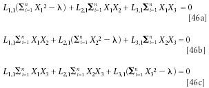
The trivial solution to equations 46a–46c still exists; setting L_1,1 = L_2,1 = L_3,1 = 0 still satisfies the three equalities. But equations 46a–46c have something that equation 34 didn't have: they have λ subtracted from the three terms corresponding to the variances of each of the variables, corresponding to the diagonal terms of the matrix [X]. This difference between the equations (46 and 34) opens the possibility that there might be another, nontrivial, solution to the equations, for a suitable value or values of λ. The original matrix [X] in equation 34 has only elements involving data values X in the matrix; therefore, the properties of the matrix are fixed by the data. Equation 46 has the extra variable λ in the equivalent matrix of X values, and thus creates the possibility that another solution exists and has the properties we are seeking, if we can find the values of λ necessary.

There are two ways to find the solutions to equations 46a–46c. One method of solving them gives a solution in closed form, leading to theoretically exact results. On the other hand, it doesn't give all the results; it allows us to find the values for λ that satisfy the equations, but not the values of L, which represent the actual functions giving the least-squares solution. Thus, it isn't a complete solution.

The other solution gives values for both λ and L. This solution, however, cannot be solved in closed form; it requires a computer-intensive computation that approximates L, and that is iterated to give better and better approximations. This makes it an open-form solution. We will start the process of finding the solutions to equations 46a–46c with the closed-form solution.

If a solution to equations 46a–46c exists, then, since the L_i are not all zero, the following equalities must hold (inspection of the matrix formulation following equation 44, ([X]^T [X] – λ[1]) { [L], makes this much clearer, that if one of the terms (the one involving L) doesn't equal zero, then the other one must equal zero, in order for the expression to equal zero). Therefore, since for a nontrivial solution to exist, [L] must not equal zero, we conclude that the term ([X]^T [X] – λ[1]) must equal zero. Converting this back into algebraic notation:

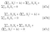
(Note: In matrix notation, equations 47a–47c become [X]^T [X] – λ[1] = [0])

Now, if you thought that the setting up of equations 47a–47c was complicated, hold on to your hat, because this is where things really start to get rolling. So fasten your seat belts, because now the ride really gets bumpy!!

Solving for λ seems easy enough. For example, we can solve for λ from equation 47a and obtain

and we could obtain similar but different formulas from equations 48b and 48c, obtaining three values for λ. The difficulty is that each of these solutions is unique only to the equation it was obtained from, and is not a solution to the other two. As we will see, there are in fact three solutions to equations 48a–48c. But since there is only one and the same λ in the three equations, any value that λ takes on must satisfy all three equations simultaneously.

Surprisingly enough, however, we already know just about everything we need to know in order to solve equations 48a–48c; believe it or not, we learned it way back when we were taking algebra. The problem is that we've forgotten it all, and never thought that we'd ever need to know it again in our lives. And ordinarily we wouldn't, except now we've taken an interest in advanced math, and the "real" mathematicians never forget these things. And you'll know exactly what I mean at the mention of one key word, which will happen in due course, when the time comes, and at the appropriate point. At which point you will all slap your heads and say things like "oh, of course!", after it all sinks in.

So let's skip to the bottom line here; later we'll come back and fill in some of the holes. This might make the ride a little more bumpy than it might otherwise be, but this way we'll at least see where we're going. The alternative is to get lost in the nitty-gritty of all the details we need to plow through, and lose sight of what our goal is.

So let's start: from advanced calculus we learn that a system of equations such as equations 48a–48c has associated with it another equation, called the "characteristic equation" (5). The characteristic equation is found from the (and here comes the magic word:) determinant (remember that from algebra? If you've forgotten, there's also a brief presentation in a previous column [6]) of the set of equations to be solved. If equations 47a–47c (which we can write in matrix notation as ([X]^T [X] – λ[1]), for simplicity) have a nontrivial solution, then the determinant of the equations, which can be written as |[X]^T [X] – λ[1]| (recall the use of the symbols "| |" as the symbols that signify the delimiters of a determinant) must equal zero (7).

It turns out, however, that we don't need advanced calculus to demonstrate this. As we will see, everything we need to know we already knew; it can all be found from elementary algebra (surprised?). Here's some more terminology from algebra that you probably forgot, just like we did: a set of algebraic equations is termed homogeneous if the constant on the right-hand side of the equations is zero, the situation we have in equations 47a–47c. For a system of homogeneous equations to have a solution other than the trivial solution, the determinant of the system of equations must be zero. Those algebra books don't tell you how to find the nontrivial solutions, however; for that you do need to go to the calculus texts. Nevertheless, the fact that having a determinant equal to zero is the condition for nontrivial solutions to exist is a result taken from fairly elementary algebra; I looked it up in reference 8, but it would be covered in almost any algebra text that discusses determinants.

In ordinary algebraic equations, the determinant of a system of equations is a single number. In a system of equations like equations 48a–48c, once all the X's are measured, the result would also be a single number, except for one difference: the equations contain the extra variable λ. However, we can still write out equations 48a–48c, and take their determinant, as they stand.

Ordinarily, a system of equations like equation 48 has either the trivial solution (all elements zero) or it can have nontrivial solutions. If there are any nontrivial solutions, then there are infinitely many of them. This is similar to the situation we saw previously in equation 34 (3). In our case, this is not an issue, because we are not looking for the general solutions to equation 48. We want to find a solution that makes the determinant of equations 48a–48c be zero.

The same algebra text (8) discusses the evaluation of determinants. While generally considered too computationally intensive for routine use on large arrays, the universally applicable method of evaluating determinants is to expand the determinant in minors (more forgotten terminology?); the minor of any given element in an array (like equation 49, for example) is the determinant of the array left after the row and column containing the selected element are deleted. The determinant of equation 49, for example, can be evaluated by expanding in minors about the first row, thusly: minors about the first row, thusly:

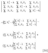
Thus, the evaluation of the 3×3 determinant is broken down into the evaluation of three 2×2 determinants. A 2×2 determinant (say, the one in the first term of equation 50) is evaluated thusly:

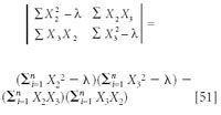
Expanding the right-hand-side of equation 51, we get

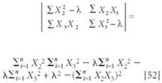
We can simplify equation 52 somewhat:

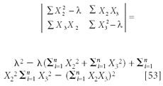
The critical point to note about equation 53 is that it is a polynomial in λ, being a quadratic in λ. The other two 2×2 determinants in equation 50, when expanded, also become formulas that are quadratic in λ. This polynomial is known as what we mentioned above: the characteristic equation of the determinant.

Now we draw your attention back to the complete first term on the right-hand-side of equation 50:

The 2×2 determinant in this term, when expanded, has a term that contains λ² (from equation 53), this is multiplied by a factor that also contains λ. In equation 53, we've shown that the 2×2 determinant expands into a quadratic polynomial in λ; therefore, the full expression becomes

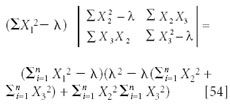
So if we multiply out the right-hand side of equation 54, we find that from the last term of the first factor, which is λ, and the first term of the second factor, which is λ², the full expansion of the 3×3 determinant contains a term with λ raised to the third power.

Therefore, the full expansion of the first term in equation 50 is a formula that is cubic in λ. Note the progression: the characteristic equation for the 2×2 determinant contains terms quadratic in λ, and the characteristic equation for a 3×3 determinant contains terms that are cubic in λ. As one might expect, the progression continues. The characteristic equation for an nth order determinant, when expanded, becomes a formula that is a polynomial, of degree n in λ.

Another rule we have learned from algebra is that a polynomial has as many roots as the highest degree term in the polynomial. In the case of determinant representing the system of equations 50, the highest exponent is three; therefore, there are three solutions to the polynomial of equation 54, and therefore three values of λ that satisfy these equations, as we described earlier in the column.

If the original data set had four variables, the same mathematical development would result in an equation corresponding to equation 50 that would contain a 4×4 determinant. To evaluate this determinant, it would have to be expanded in minors; this would result in four 3×3 determinants, each of which would expand into three 2×2 determinants, or 12 2×2 determinants altogether. Having done so, however, we would then arrive at a quartic equation for the characteristic equation.

Five variables in the data would expand into 60 2×2 determinants, giving rise to a quintic polynomial for the characteristic equation, and so forth: the amount of computation needed to evaluate an m×m determinant expands factorially as m increases. Thus, while useful for explaining what is going on "under the hood," this method quickly becomes impractical as a means of actually arriving at a solution to the original problem, even with computers. To give some full disclosure here, there are procedures that can reduce the amount of computation, and for the higher-order determinants the savings becomes appreciable. Nevertheless, the amount of computation needed would still expand exponentially, even though not factorially, in that case, so this is still not a practically useful way to actually solve the equations.

Solving polynomial characteristic equations is another topic that, like determinants, is covered in the (fairly elementary) algebra courses that we all took (no matter how much we've forgotten them!) and therefore, once-upon-a-time, we did in fact know how to do them. For this reason, we will not be describing them here; when you want to know the details, you can go back and study what you once knew, just like I did.

The solution of the polynomial described in equation 54 provides the values for λ that solve equations 47a–47c, or at least allow the left-hand side of the equations to be zero; even though for those values of λ there will be infinitely many solutions. However, we have yet to determine the functions corresponding to those roots, that is the least-square estimator. In the next installment of this column, therefore, we will see how to narrow those solutions down to the ones that give us finite results that are the solutions to the original problem of finding the maximum-variance approximation of the original data set [X] (we've got to keep track of where all this is heading, you know).

Jerome Workman, Jr. serves on the Editorial Advisory Board of Spectroscopy and is currently with Luminous Medical, Inc., a company dedicated to providing automated glucose management systems to empower health care professionals.

Howard Mark serves on the Editorial Advisory Board of Spectroscopy and runs a consulting service, Mark Electronics (Suffern, NY). He can be reached via e-mail: hlmark@prodigy.net

References

(1) H. Mark and J. Workman, Spectroscopy 22(9), 20–29 (2007).

(2) H. Mark and J. Workman, Spectroscopy 23(2), 30–37 (2008).

(3) H. Mark and J. Workman, Spectroscopy 23(5), 14–17 (2008).

(4) H. Mark and J. Workman, Spectroscopy 23(6), 22–24 (2008).

(5) A.E. Taylor, Advanced Calculus (Ginn and Company, New York, New York, 1955).

(6) J. Workman and H. Mark, Spectroscopy 9(4), 18–19 (1994).

(7) D. Zwillinger, CRC Standard Mathematical Tables and Formulae (Chapman & Hall/CRC Press, New York, New York, 2003).

(8) W.L. Hart, Brief College Algebra (D.C. Heath & Co., Boston, Massachusetts, 1947).