Corrections to Analysis of Noise: Part I

We occasionally get feedback from our readers. Often, the feedback is positive, letting us know that they find reading these columns interesting, enjoyable, and most importantly, useful. Getting responses like that also makes writing these columns interesting and enjoyable, and makes us feel useful, too. Occasionally, one or more readers finds an error (horrors!) that requires a correction (more horrors!), or presents an alternative approach to, or interpretation of, our discussion. When we wrote our 14-part column on the analysis of noise in spectroscopy, a few readers wrote in, letting us know that they felt that some parts of the derivations were weak, and perhaps less than perfectly rigorous. We took their comments to heart and here present the first of a two-part discussion incorporating the comments. This could be considered a (hide your eyes!) correction, or perhaps, simply another approach to analyzing the situation.

Some time ago, we published a subseries of columns within this series (1–14) giving rigorous derivations for the expressions relating the effect of instrument noise and other types of noise to their effects on the spectra we observe. During and after the publication of those columns, we received several comments discussing various aspects, including some errors that crept in. Most of those were minor and can be ignored (for example, a graph axis labeled "Transmission" when the axis went from 0–100%, and therefore, the axis should have been labeled "% Transmission").

Jerome Workman, Jr.

One comment, however, was a little more significant, and therefore, we need to take cognizance of it. One of our respondents noted that the analysis performed could be done in a different way, a way that might be superior to the way we did it. Normally, if we agree with someone who takes issue with our work we would simply publish a correction (assuming their comments are persuasive). In this case, however, that seems inappropriate for several reasons. First, the original analysis was published a long time ago and cannot be dispensed with easily. Second, we're not convinced that our original approach is wrong; therefore, it is not clear that a correction is warranted. Third, some of our readers might wish to compare the two approaches for themselves to decide if the original one is actually wrong or simply not as good, or whether, in fact, the new analysis is better. Therefore, we present a new, alternate analysis, along the lines recommended by our respondent.

Howard Mark

Alternate Analysis

The point of departure is from our original column (5), which dealt with the effect of random, normally distributed noise whose magnitude (in terms of standard deviation) is independent of the strength of the optical signal. Here we present the revised analysis of this situation of the effect on the expected noise level of the computed transmittance when the signal noise is not small compared to the signal level E_r.

Before we proceed, however, there is a technical point we need to clear up, and that is the numbering of the equations in this column series. Ordinarily, when continuing a subject through several columns, we simply continue the numbering of equations as though there were no break. The column representing our point of departure ended with equation 63. Therefore, it is appropriate to begin this alternate analysis (5) with equation 64, as we would normally. However, equation number 64 (and subsequent numbers) was already used; therefore, we cannot simply repeat using the same equation numbers that we used already. Neither can we simply continue from the last number used in the original analysis (5) because they would also conflict with the equation numbers already used for other purposes.

We resolved this dilemma by adding the suffix "a" to the equation numbers used in this column. Therefore, the first new equation we introduce here will be equation 64a. Fortunately, none of the equations developed in the column with the original analysis, nor the figures, used any suffix, as was done occasionally in other columns (we will copy equation 52b from the previous column, but the "b" suffix does not signify a new equation because it is the equation used previously; also, a "b" suffix is not indicative of a copy of an equation number here, only an "a" suffix). Therefore, we can distinguish the numbering of any equations or other numbered entities in this section by appending the suffix "a" to the number without causing confusion with other corresponding entities.

Now we are ready to proceed.

We reached this point from the discussion just before equation 64 (5). A reader of the original column felt that equation 64 was being used incorrectly. Equation 64, of course, is a fundamental equation of elementary calculus and is itself correct. The problem pointed out was that the use of the derivative terms in equation 64 implicitly indicates that we are using the small-noise model, and especially when changing the differentials to finite differences in equation 65, results in incorrect equations.

In our previous column (4), we had created an expression for T + ΔT (as equation 51) and separated out an expression for ΔT (as equation 52b). We present these two equations here:

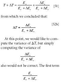
will vary due to the presence of the ΔE_r in the denominator, and using only the second term would ignore the influence of the variability of the first term in equation 51 (4) and not take its contribution to the variance into proper account. Therefore, the expression for ΔT in equation 52b is not correct, even though it is the result of the formal breakup of equation 51 (4). We should be using a formula such as the following:

to include the variability of the first term, also.

This, however, leads to another problem: subtracting equation 64a from equation 51 leaves us with the result that T = 0. Furthermore, the definition of T gives us the result that E_s is zero, and that therefore, ΔT is in fact equal to the expression given by equation 52b anyway despite our efforts to include the contribution to the variance of the first term in equation 51.

Our conclusion is that the original separation of equation 51 into two equations, while it served us well for computing T_M and T_A, fails us here when computing the variance of the transmittance. This is because ΔE_s and ΔE_r are random variables and we cannot treat their influences separately; we have no expectation that they either will cancel or reinforce each other, wholly or partially, in any particular measurement. Therefore, when we compute the variance of ΔT, we need to retain the contribution from both terms.

This also raises a further question: the analysis of equation 52a by itself served us well, as we noted, but was it proper, or should we have maintained all of equation 51, as we find we must do here? The answer is yes, it was correct, and the justification is given toward the end of the earlier column (4). The symmetry of the expression when averaged over values of E_s means that the average will be zero for each value of E_r, and therefore, the average of the entire second term will always be zero.

Therefore, we conclude that the best way to maintain the entire expression is to go back to a still earlier step and note that the ultimate source of equation 51 was equation 5 (2):

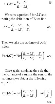
Because E_s/E_r is the true transmittance of the sample, the value of T for a given sample is constant, and the variance of that term is zero, resulting in equation 68a:

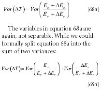
that would not be correct because the two variances that we want to add have a common term (E_r + ΔE_r), and therefore, are not independent of each other as application of the rule for adding variances requires (2). Also, evaluation of a variance by integration requires the integral of the square of the varying term, which as we have seen previously (5), is always positive, and therefore, the integrals of both terms of equation 69a diverge.

Thus, we conclude that we must compute the variance of ΔT directly from equation 68a and the definition of variance:

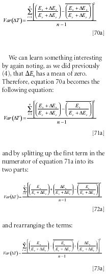
and again using the definition of variance:

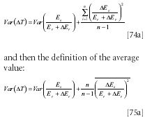
where we note that the limit of n/(n - 1)→ 1 as n becomes indefinitely large. Of course, the noise level we want will be the square root of equation 75a.

We have seen previously, in equation 77 (5), that the variance term in equation 75a diverges, and clearly, as ΔE_r → –E_r, the second term in equation 75a also becomes infinitely large. However, as we discussed at the conclusion of the original analysis, using finite differences means that the probability of a given data point having ΔE_r close enough to –E_r to cause a problem is small, especially as E_r increases. This allows for the possibility that a finite value for an integral can be computed, at least as long as E_r is sufficiently large.

To recapitulate some of that here, it was a matter of noting two points: first, that as E_r gets further and further away from zero (in terms of standard deviation), it becomes increasingly unlikely that any given value of ΔE_r will be close enough to E_r to cause trouble. The second point is that, in a real instrument there is, of necessity, some maximum limit on the value that 1/(E_r – ΔE_r) can attain, due to the inability to contain or represent an actually infinite number. Therefore, it is not unreasonable to impose a corresponding limit on our calculations, to correspond to that physical limit.

We now consider how to compute the variance of ΔT, according to equation 68a. Ordinarily, we would first discuss converting the summations of finite differences to integrals, as we did previously, but we will forbear that, leaving it as an exercise for the reader. Instead, we will go directly to consideration of the numerical evaluation of equation 68a, because a conversion to an integral would require a back-conversion to finite differences in order to perform the calculations.

We wish to evaluate equation 68A for different values of E_s and E_r when each is subject to random variation. Note that Var (ΔE_s) = Var (ΔE_r). We cannot simply set the two terms equal to a common generic value of ΔE, as we did previously, as that would imply that the instantaneous values of ΔE_s and ΔE_s were the same. But of course they're not, because we assume that they are independent noise contributions, although they have the same variance. Under these conditions, it is simplest to work with equation 68a itself, rather than any of the other forms we found it convenient to convert equation 68a into, for the illustrations of the various points we presented and discussed.

There are still a variety of ways we can approach the calculations. We could assume that E_s or E_r were constant and examine how the noise varies as the other was changed. We could also hold the transmittance constant and examine how the transmittance noise varies as both E_s and E_r are changed proportionately.

What we will actually do here, however, is all of these. First, we will assume that the ratio of E_s/E_r, representing T, the true transmittance of the sample, is constant, and examine how the noise varies as the signal-to-noise ratio (S/N) is changed by varying the value of E_r, for a constant noise contribution to both E_s and E_r. The noise level itself, of course, is the square root of the expression in equation 67a:

To do the computations, we again use the random number generator of MATLAB to produce normally distributed random numbers with unity variance to represent the noise. Values of E_r will then directly represent the S/N of the data being evaluated. For the computations reported here, we use 100,000 synthetic values of the expression on the right-hand side of equation 76a to calculate the variance, for each combination of conditions we investigate.

Figure 1

A graph of the transmittance noise as a function of the reference S/N is presented in Figure 1a and the expanded portion of Figure 1a, shown in Figure 1b. The "true" transmittance, E_s/E_r was set to unity (that is, 100% T).

The inevitable existence of a limit on the value of T_M, as described in the section following equation 75a, was examined in Figure 1a by performing the computations for two values of that limit, by setting the limit value (somewhat arbitrarily, to be sure) to 1000 and 10,000, corresponding to the lower and upper curves, respectively.

Note that there are effectively two regimes in Figure 1a, with the transition between regimes occurring when the value of S/N equals approximately 4. When the value of E_r was greater than approximately 4 — that is, S/N was greater than four — the curves were smooth and appear to be well behaved. When E_r was below S/N of 4, the graph entered a regime of behavior that shows an appreciable random component. The transition point between these two regimes would seem to represent an implicit definition of the "low noise" versus the "high noise" conditions of measurement. In the low-noise regime, the transmittance noise decreases smoothly and continuously as S/N increases. This was verified by other graphs (not shown) that extended the value of S/N beyond what is shown here.

The "high-noise" regime seen in Figure 1a is the range of values of S/N in which the computed standard deviation is grossly affected by the closeness of the approach of individual values of ΔE_r to E_r. This is, in fact, a probabilistic effect, because it not only depends upon how closely the two numbers approach each other, but also on how often that occurs; a single approach or only a few "close approaches" will be lost in a large number of readings where that does not happen. As we will see, there is indeed a regime in which the theoretical "low-noise" approximation differs from the results we find here, without becoming randomized.

Changing the number of values of (E_s + ΔE_s)/(E_r + ΔE_r) used for the computation of the variance made no difference in the nature of the graph. As is the case in Figure 1a, the transition between the low- and high-noise regimes continues to occur at a value between approximately 4 and 5.

Figure 2 shows the graph of transmittance noise computed empirically from equation 76a, compared to the transmittance noise computed from the theory of the low-noise approximation, as per equation 19 (2) and the approach, under question, of using equation 52b. We see that there is a third regime, in which the difference between the actual noise level and the low-noise approximation is noticeable, but the computed noise has not yet become subject to the extreme fluctuations engendered by the too-close approach of ΔE_r to E_r. Because the empirically determined curve will approach the theoretical curve asymptotically as S/N increases, where the separation becomes "noticeable" will depend, apparently, on how hard you look.

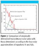
Figure 2

We also observe that the approximation of using equation 52b gives a proper qualitative description to the behavior of the noise, but in the low-noise regime, a quantitative assessment appears to give noise values that are low by a factor of roughly two.

We will continue our discussion in the next column.

Jerome Workman, Jr. serves on the Editorial Advisory Board of Spectroscopy and is director of research and technology for the Molecular Spectroscopy & Microanalysis division of Thermo Fisher Scientific. He can be reached by e-mail at: jerry.workman@thermo.com

Howard Mark serves on the Editorial Advisory Board of Spectroscopy and runs a consulting service, Mark Electronics (Suffern, NY). He can be reached via e-mail: hlmark@prodigy.net

References

(1) H. Mark and J. Workman, Spectroscopy15(10), 24–25 (2000).

(2) H. Mark and J. Workman, Spectroscopy15(11), 20–23 (2000).

(3) H. Mark and J. Workman, Spectroscopy15(12), 14–17 (2000).

(4) H. Mark and J. Workman, Spectroscopy16(2), 44–52 (2001).

(5) H. Mark and J. Workman, Spectroscopy16(4), 34–37 (2001).

(6) H. Mark and J. Workman, Spectroscopy16(5), 20–24 (2001).

(7) H. Mark and J. Workman, Spectroscopy16(7), 36–40 (2001).

(8) H. Mark and J. Workman, Spectroscopy16(11), 36–40 (2001).

(9) H. Mark and J. Workman, Spectroscopy16(12), 23–26 (2001).

(10) H. Mark and J. Workman, Spectroscopy17(1), 42–49 (2002).

(11) H. Mark and J. Workman, Spectroscopy17(6), 24–25 (2002).

(12) H. Mark and J. Workman, Spectroscopy17(10), 38–41, 56 (2002).

(13) H. Mark and J. Workman, Spectroscopy17(12), 123–125 (2002).

(14) H. Mark and J. Workman, Spectroscopy18(1), 38–43 (2003).