The Long, Complicated, Tedious, and Difficult Route to Principal Components: Coda

As we usually do, when we continue the discussion of a topic through more than one column, we continue the numbering of equations from where we left off.

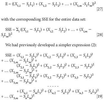
At this point, we have already solved the main problem, but a nagging question comes to mind. In computing the sum-squared-error (SSE), we used the following expression for the squared error (1):

and found that it gave only the trivial solution. At that time, we had not yet introduced the use of Lagrange multipliers, so the natural question that comes to mind at this point is, what would have happened if we had used the simpler expression for the SSE, and applied the same constraint that the sum of the squares of the coefficients had to equal a constant (unity) to that?

Let's make the same simplification of notation we did previously and follow through with this development. Simplifying equation 19 by using only three variables worth of data, redefining the error matrix to represent the variance accounted for, and using only the variance terms of equation 19, the expression for SSE becomes

(where A, from the simplified form of equation 19, represents the total accounted-for difference between the principal component and the date, and SSA is the sum-squared accounted-for difference, corresponding to equation 28).

Then the corresponding expression for SSA becomes:

Note the absence of cross-terms (that is, X_iX_j). This development of the equations does not create the covariance terms that were present in the equations leading to the final solution. We will see shortly that this has significant consequences.

We now introduce the constraint L_1,1² + L_2,1² + L_3,1² = 1 with the Lagrange multiplier, as we did before:

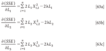
Again we take derivatives with respect to the various L_i:

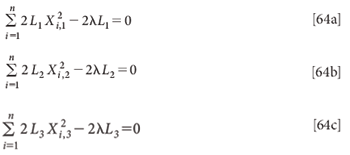
Setting these derivatives equal to zero:

Again, the trivial solution L₁ = L₂ = L₃ = 0 exists. Do these equations have any nontrivial solutions, as we found for the multivariate case? We can examine these equations according to the same approach that we used for the multivariate solution (3).

Then, as with the multivariate case, we can solve the individual parts of equations 64 for λ, in the case of equation 64a we find

but again, we find that this solution is good only for equation 64a. Equation 64b requires the following solution:

and equation 64C has the following solution:

This is where our attempt must terminate. The next step we took to solve the equations was to set up a determinant. Here we do not have the connection between the equations that we had in the multivariate case, and we cannot set up the determinant that might lead to a characteristic equation that was a polynomial in λ, as we did previously. Indeed, equations 63 do not even really constitute a system of equations, they are merely three separate, distinct, and independent equations; there are no connections between them, as we had in equations 46, where the cross-terms connected the equations due to the fact that they represented the same variables.

Thus ends false start 3.

And thus ends our analysis of principal components..

Howard Mark serves on the Editorial Advisory Board of Spectroscopy and runs a consulting service, Mark Electronics (Suffern, NY). He can be reached via e-mail: hlmark@prodigy.net

Howard Mark

Jerome Workman, Jr. serves on the Editorial Advisory Board of Spectroscopy and is currently with Luminous Medical, Inc., a company dedicated to providing automated glucose management systems to empower health care professionals.

Jerome Workman, Jr.

References

(1) H. Mark and J. Workman, Spectroscopy 23(5), 14–17 (2008).

(2) H. Mark and J. Workman, Spectroscopy 23(2), 30–37 (2008).

(3) H. Mark and J. Workman, Spectroscopy 23(10), 24–27 (2008).