Optimizing the Regression Model: The Challenge of Intercept–Bias and Slope “Correction”
Spectroscopy
The archnemesis of calibration modeling and the routine use of multivariate models for quantitative analysis in spectroscopy is the confounded bias or slope adjustments that must be continually implemented to maintain calibration prediction accuracy over time. A perfectly developed calibration model that predicted well on day one suddenly has to be bias adjusted on a regular basis to pass a simple bias test when predicted values are compared to reference values at a later date. Why does this problem continue to plague researchers and users of chemometrics and spectroscopy?
The archnemesis of calibration modeling and the routine use of multivariate models for quantitative analysis in spectroscopy is the confounded bias or slope adjustments that must be continually implemented to maintain calibration prediction accuracy over time. A perfectly developed calibration model that predicted well on day one suddenly has to be bias adjusted on a regular basis to pass a simple bias test when predicted values are compared to reference values at a later date. Why does this problem continue to plague researchers and users of chemometrics and spectroscopy?
The subject of bias and slope, also known as intercept and slope adjustments, following calibration transfer has been an integral part of the application of multivariate calibrations since the very beginning. It is well understood, and widely accepted, that following the transfer of multivariate calibrations from one instrument to another there is a bias adjustment required for the predicted results to conform to the reference values from a set of reference transfer samples. There have been many attempts to reduce this bias or intercept requirement, but the fact remains that intercept and slope are routinely used for calibration transfer from one instrument to another.
One may derive a number of explanations for the requirement for intercept or slope adjustments following calibration transfer. One reason often given is that laboratory values differ. This may be true in some cases, but is completely irrelevant to the issue that if one transfers a calibration from one identical instrument to another the predicted values should be identical for the same sample set from one instrument to another (within normal statistical variation). This brings us to the key point of discussion for this column.
If one will engage in a gedankenexperiment with us, momentarily one can conceive of a time and technology where intercept and slope will not be required for one instrument to produce identical results to another instrument following calibration transfer. In this thought experiment let us conceive of instrumentation that is precisely alike in spectral shape from one instrument to another when measuring an identical sample. For such an instrument, the predicted values using the same calibration equation across instruments will give precisely the same results. We have discussed this issue in the past and demonstrated that when using near-infrared (NIR) spectrophotometers for predictions, even if one uses random numbers for the dependent variables (representing the reference or primary laboratory results), that different instruments will closely predict these random numbers across instruments following calibration transfer. Thus, the instrument could be considered agnostic in terms of the numbers it generates using a spectral measurement when combined with multivariate calibration equations (1).
We have also pointed out in the past some of the various requirements for successful calibration transfer and the wide differences between commercial instruments in terms of agreement for wavelength and photometric axes registration (2-7). Furthermore, we have reminded ourselves that spectrophotometers using Beer’s law (and even Raman spectrometers that “self determine” pathlength) measure moles per unit volume or mass per unit volume and do not measure odd or contrived reference values simply by adding more terms to the regression model (8,9). Note that irrespective of the chemometric approaches used to develop a calibration model, an inconsistent spectral shape with changing x- and y-axis registrations over time, and between instruments, will disrupt any model such that the intercept and slope corrections remain a requirement following calibration transfer. Readers are also reminded that calibration models that accommodate too much wavelength and photometric variation within the data lose significant predictive accuracy. So, to return to our thought experiment, we are imagining that all instruments are identical using a new form of manufacturing technology and that we are able to measure the same set of samples on a series of such spectrophotometers and use the same identical calibration equation to obtain the same identical predicted results from each instrument without the need for any bias and slope adjustments.
Note that the entire issue for relating the spectra from each instrument to specific reference laboratory results is immaterial for this discussion, since given any instrument the identical results will be obtained. One must obviously decide what chemical parameters and reference laboratory to use to provide the correct reference values relative to any individual sample. As a reminder, this should be reported as weight or mass per volume and not weight percent or other contrived values if one wants to better relate the spectroscopy to the reported predicted values.
Now, there are many issues associated with making instruments alike enough to eliminate the bias and slope problem. This column installment is intended to begin a discussion on the issues involved and to surface some of the mathematical and engineering approaches intended to move toward correcting any instrument differences. The technology will certainly arise at some point to eliminate this problem, so let us move in that direction and begin addressing the issues. We remind the reader that we will refer to no metaphysics; only standard physics and statistics are involved.
So, what are the main differences between instruments that cause the slope and intercept challenges related to calibration transfer? We discuss three of these differences here and hopefully more fully address these and other issues in some future columns. For this article let us discuss: wavelength shift (x-axis), photometric shift (y-axis), and linewidth or lineshape (spectral resolution and shape) as the primary causes of the intercept and slope variation between instruments following calibration transfer. Note that these authors have expounded on the intuitive problem of having a fixed calibration model for use with a dynamic instrument condition in previous publications. Either the calibration must become dynamic to compensate for instrument changes or the instrument must be corrected to a constant initial state if a fixed model is to be applied with consistent predictive results.
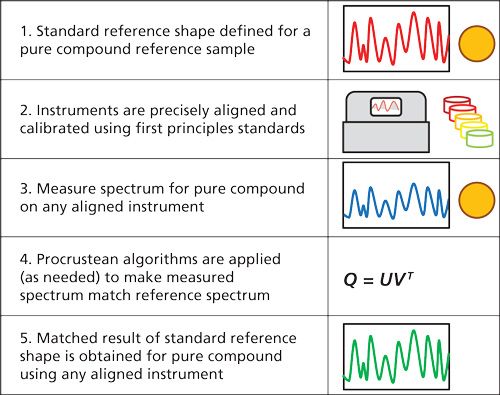
As we continue discussion with our thought experiment, one could envision a time when the spectrum of a pure compound could be defined in such a way that given a specific spectral resolution, one would define a standard reference spectrum of a pure compound. The further expectation would be that all properly aligned and calibrated spectrophotometers would be expected to produce an identical spectrum from the same sample of the pure compound. Such a future technology would require instrumentation to be precisely calibrated using first principles physical standards with a predefined linewidth and lineshape. These aspects would be combined with a series of Procrustean algorithms to conform a measured result to a precise reference result. One may see this as a multistep process resembling Figure 1.
So, along these lines of our thought experiment, let us now examine some of the issues associated with the challenge of instrumental differences that cause calibration transfer slope and intercept woes. Such primary instrument differences include wavelength shift, photometric shift, and linewidth or lineshape changes. These are the primary causes for intercept and slope changes between instruments used for calibration transfer.
To demonstrate the effects of changes in wavelength, photometric, and line-width or lineshape parameters in principle, and to demonstrate the mathematics used to compute the confidence limits associated with comparing standard error, intercept (bias), and slope we present a simple univariate regression case with a single near Gaussian spectral band. For this demonstration, we examine the effects of shifting or altering the spectral band on the predicted results when applying the original univariate calibration equation (10).
The Initial Spectra and Calibration Equation
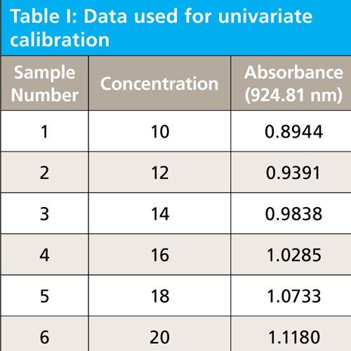
A set of six spectra are derived having a single near symmetrical Gaussian band representing six concentrations of analyte. The spectra and data table are given as Figure 2, and Table I, respectively. The linear regression, formed at 924.81 nm peak maximum, from this data results in the univariate linear regression equation 1. This equation will be applied to all spectra after they have been altered to test the effect of the various alterations upon the predicted results. A summary of results and a discussion section will be presented at the conclusion of this column.
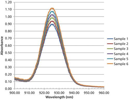
Figure 2: Simulated spectral data used for univariate calibration (six samples).

Changing the Wavelength Registration
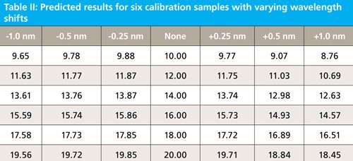
In the first experiment, we shift wavelength registration by -1.0 nm, -0.5 nm, -0.25 nm, and +0.25 nm, +0.50 nm, and +1.0 nm. From testing commercial NIR instrumentation these differences would be expected between manufacturers. When the wavelength registration is changed by these amounts the resulting spectra and prediction results are as follows in Figure 3, and Table II.
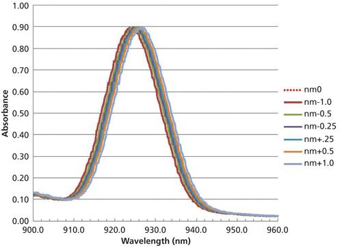
Figure 3: A single spectral band from one sample (sample 1) shifted by different wavelength amounts; the unshifted spectrum is represented by the dotted red line.
Changing the Photometric Registration
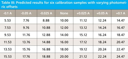
In the second experiment we shift photometric registration by -0.1 A, -0.05 A, -0.025 A, no shift, and +0.025 A, +0.05 A, and +0.1 A. These would be typical differences expected between manufacturers or even within the same instrument over time. When the photometric registration is changed by these amounts the resulting spectra and prediction results are as follows in Figure 4, and Table III.
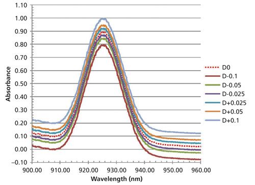
Figure 4: A single spectral band from one sample (sample 1) shifted by different photometric offset amounts; the unshifted spectrum is represented by the dotted red line.
Changing the Linewidth or Lineshape
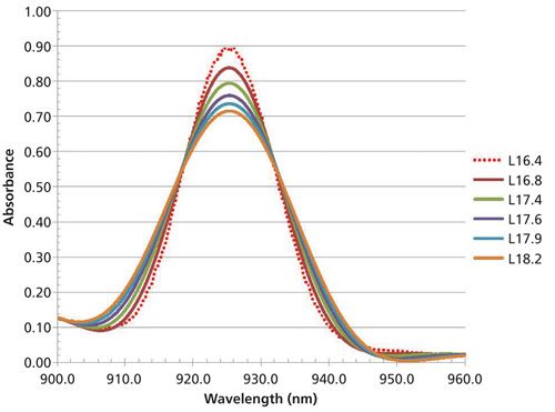
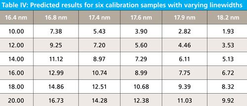
In the third experiment, we change the linewidth as full width at half maximum (FWHM) to have values of 16.4, 16.8, 17.4, 17.6, 17.9, and 18.2 nm. These would be typical changes expected between manufacturers or even within the same instrument design criteria over severe differences in manufacturing iterations with new model designs. When the linewidth is changed by these amounts the resulting spectra and prediction results are as follows in Figure 5, and Table IV. Note that as the bandwidth changes, the amplitude also changes.
Discussion and Review of Results
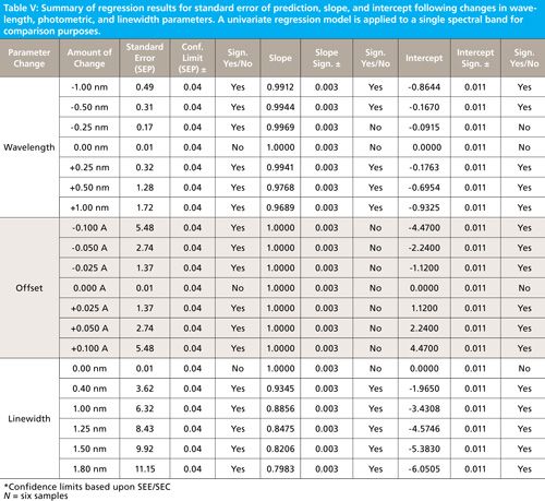
Table V summarizes results from these experiments. For each parameter tested (that is, the standard error of prediction, the slope, and the intercept) the confidence limits and significance decisions are given in separate columns. The equations for computing the confidence limits for each statistical parameter (that is, predicted values, slope, and intercept) are given in equations 2 through 6.
Confidence Limits for Predicted Values from a Regression
To compute the upper and lower confidence limits for any predicted value, the following equations 2 and 3 are used. First compute the standard error of calibration (SEC)-this is 0.01 for our example. The SEC is computed as shown in equation 2.

For this equation n is the number of calibration samples; k is the number of wavelengths (or factors) used for the initial calibration; yi is the reference laboratory results for each ith sample; and Å·i is the predicted results for each ith sample.
The confidence limit for the predicted value is then computed as shown in equation 3 (11).

Where CLŶ indicates the confidence limits for the predicted value based on the standard error of calibration, the t value is for n - k - 1 degrees of freedom, and the Mahalanobis distance (D) of the predicted sample is used. For this simulation one may substitute 0 or 1 for the D value. In our example case, t = 2.78 for n - 2 = 4 degrees of freedom and 95% confidence for a two-tailed α = 0.05 test. The predicted value confidence limit is posted within Table V, indicating that all changes had a significant effect on the predicted values. The confidence limit for any predicted value is computed to be ±0.04 for our example.
Confidence Limits for Slope from a Regression
The confidence limits for the slope of a regression are computed as shown in equations 4 and 5. First we compute the standard error of the slope as shown in equation 4.
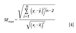
For this equation n is the number of calibration samples; xi is the reference laboratory results for each ith sample; and xi is the mean reference value for all samples, that is, the mean concentration value. So yi is the dependent variable; xi the independent variable; and n is the number of samples. Note: yi and Å·i are as in equation 2.
The confidence limit for the slope of the regression line is then computed as shown in equation 5.

Where CLslope gives the confidence limits for the slope value based on the standard error of the slope, the t value is for n - 2 degrees of freedom. For this example, t = 2.78 for n - 2 = 4 degrees of freedom and 95% confidence for a two-tailed α = 0.05 test. The slope confidence limit is posted within Table V indicating that offset and a slight wavelength shift of -0.25 nm have no effect on the slope value; all other changes had a significant effect on the slope values. The confidence limit for the slope is computed to be ±0.003 for our example.
Confidence Limits for Intercept or Bias from a Regression
The confidence limits for the intercept or bias of a regression are computed as shown in equations 2 and 6. First we compute the standard error of a validation set or alternatively the standard error of the calibration as shown in equation 2. The confidence limit for the intercept or bias value is then computed as shown in equation 6.

Where CLintercept gives the confidence limits for the intercept value based on the standard error of calibration or prediction, the t value is for n -2 degrees of freedom. For our example case, t = 2.78 for n - 2 = 4 degrees of freedom and 95% confidence for a two-tailed α = 0.05 test. The intercept confidence limit is posted within Table V indicating that all effects (other than a -0.25 nm wavelength shift) had a significant effect on the intercept values. The confidence limit for the intercept is computed to be ±0.011 for our example.
Summary of Results
Note that in our univariate regression example that most changes to a spectrum had a serious effect on intercept and slope values, even though in this example only the peak height would change the prediction results. In the multivariate case, not only peak height but also spectral shape would have a more profound effect on predicted values. Some spectral changes may be partially mitigated by changing the intercept or bias for each prediction equation, although changing the bias does not bring the model into conformance with the spectral changes. We note that more complex multivariate calibration is partially able to compensate for some instrument differences that cause spectral changes; however, the same prediction results will not arise from intercept and slope corrections when spectra are significantly different; recalibration is a requirement when spectra are significantly different between instruments.
We note for the univariate example shown that we have demonstrated some of the issues and mathematics used to assess calibration transfer when spectral profiles are different from one instrument to another. This instrument difference problem is magnified when the specific type of instrument design is not matched, such as dispersive grating versus Fourier transform-based interferometer spectrophotometers versus diode array, and so on. This first column, demonstrating a univariate case on the subject of intercept and slope changes caused by typical instrumental differences, demonstrates the concepts and mathematics that will be explored in future discussions of this topic.
References
(1) H. Mark and J. Workman Jr., Spectroscopy22(6), 14-22 (2007).
(2) H. Mark and J. Workman Jr., Spectroscopy 28(2), 24-37 (2013).
(3) J. Workman Jr. and H. Mark, Spectroscopy 28(5), 12-25 (2013).
(4) J. Workman Jr. and H. Mark, Spectroscopy 28(6), 28-35 (2013).
(5) J. Workman Jr. and H. Mark, Spectroscopy 28(10), 24-33 (2013).
(6) J. Workman Jr. and H. Mark, Spectroscopy 29(6), 18-27 (2014).
(7) J. Workman Jr. and H. Mark, Spectroscopy 29(11), 14-21 (2014).
(8) H. Mark and J. Workman Jr., Spectroscopy 27(10), 12-17 (2012).
(9) H. Mark and J. Workman Jr., Spectroscopy 29(2), 24-37 (2014).
(10) H. Mark, Principles and Practice of Spectroscopic Calibration, 1st Ed. (Wiley, New York, 1991), pp. 7, 14, 15.
(11) ASTM E1655-05(2012), “Standard Practice for Infrared Multivariate Quantitative Analysis,” (American Society for Testing and Materials [ASTM] International, West Conshohocken, Pennsylvania, 2012).
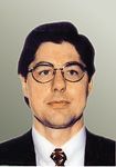
Jerome Workman Jr. serves on the Editorial Advisory Board of Spectroscopy and is the Executive Vice
President of Engineering at Unity Scientific, LLC, in Brookfield, Connecticut. He is also an adjunct professor at U.S. National University in La Jolla, California, and Liberty University in Lynchburg, Virginia. His e-mail address is: JWorkman04@gsb.columbia.edu

Howard Mark serves on the Editorial Advisory Board of Spectroscopy and runs a consulting service, Mark Electronics, in Suffern, New York. He can be reached via e-mail: hlmark@nearinfrared.com
