Quantitative Mass Spectrometry Part III: An Overview of Regression Analysis

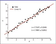
In the last column, a simplified figure portrayed the expected distribution of measurements for one selected calibration point. Any one point can be used to establish the proportionality factor between measured response and analyte amount; the range of expected measurement values means there will be a concomitant range of proportionality constants. In part to establish a useable dynamic range for our actual measurements, we typically use several calibration points, and each will produce a range of proportionality constants. Figure 1 represents the results of a linear regression analysis line fit to a number of calibration points. The dependent variable y is measured as a function of the independent variable x. This is one of the simplest forms of regression analysis, and it predicts the value of one variable from another when the relationship between them is assumed to be linear. The geometrical description of the line is of the form y = a + bx, where x is the independent variable and y is the dependent variable. The slope of the line is b (representing the best-fit proportionality constant), and a is the intercept (the value of y when x = 0). Simplistically, the goal of a regression analysis is to find those values of a and b that describe a line closest to the data. The equation given above that describes the line is a restatement of the more common form of a line equation y = mx + b. This author prefers the given form because it emphasizes that some instrumental response should be observed even in the absence of analyte; this measured value previews a determination of noise in the analytical system. The restated form of the equation also emphasizes that both a and b are variables with a range related to the confidence limits required. Thus, the values of a and b given in Figure 1 reflect the range of values.

Kenneth L. Busch

The well-behaved linear regression is a focus of the calibration section of undergraduate analytical chemistry textbooks, and the elusive goal of some of our laboratory work in quantitative analysis. Because the amount of analyte is assumed known to a high degree of accuracy (or without any error at all), this value on the x axis is considered to be an independent variable. The random errors in the measured values for the "known and fixed" amount are distributed along the vertical y axis. We begin with an overview of the term "expected." We prefer an analytical world to be simpler rather than more complex, and linear as contrasted with multivariate. In constructing analytical protocols, usually we choose to measure a dependent value directly and simply proportional to the analyte (or value) of interest, and we will modify the testing protocol to provide this linear proportionality across the range of interest. Within the constrained testing and development phase of the protocol, the simplicity and linearity of the model for the distribution of results can be confirmed. As the protocol is put into place in the real world, and experience accrues — or as the analytical milieu changes, as requisite analytical tolerances grow tighter, or even as instruments or analysts change — a previously sufficient linear model might need to be reworked and revalidated.

Figure 1: Generic appearance of a linear regression line that links observed response (y axis) to known analyte amount (x axis). The figure originally appears in reference 2.

A more sophisticated regression analysis might continue to provide useful results, but the need to invoke such a "fix" should also trigger a re-evaluation of the underlying "expected" assumptions.

What do we measure in MS that provides a response directly proportional to the amount of sample? Mass spectra plot the relative abundances of ions of various masses, and (to a pretty good approximation) the amount of sample present does not change the appearance of the mass spectrum. In a gas chromatography (GC)–MS instrument, as in the use of other detectors for GC, we could use the single-channel detector response (tabulated as the total ion current) as a measured value proportional to the amount of sample. In this approach, the "area-under-the-curve" is derived from the absolute magnitude of the total ion current. Of course, the magnitude of the total ion current is a function of the mass range scanned, and this would be kept constant in preparation of a calibration curve and analysis of samples. Because mass spectra are additive, the mass range usually scanned for organic GC–MS does not include the masses of low mass background ions such as air, argon, or carbon dioxide. Including any background ions in the total ion current summation will increase the variance of the measured results. Alternatively, we can choose as a measured response the absolute intensities of several ions of specific masses that appear in the mass spectrum of the targeted analyte. These summed intensities represent a subset of total ion current, with a value proportional to the amount of sample. The accuracy of such a quantitative determination might be enhanced because variance contributions from ions of background masses are removed from the proportionality equations. It is not necessary to include all the ions in the analyte's mass spectrum within such a summation of absolute ion current; any representative subset should provide a calibration curve of similar quality. However, it is important to include several such ions, especially at low values of the measured absolute ion current.

As described, in quantitative MS, the measured value traditionally has been the absolute intensity of an ion or group of ions. Many other measurements — both kinetic and thermodynamic in basic nature — can be completed, but these measurements are topics for future columns. In deference to the simple traditional question of how much analyte there is, the analyst almost always will be constructing a proportionality curve for calibration based upon absolute ion intensities. The analyst might select a mass range, or, as described earlier, include only ions of masses specific to the sample, or, to increase specificity and increase accuracy, include only ions specified within a narrow mass window. With use of higher resolution, sensitivity usually is traded in a balance against mass resolution. But a lower sensitivity under the usual conditions might be compensated by the use of a higher gain in the detection system, or an offsetting advantage of lower noise in the signal, such that the requisite sensitivity and desired accuracy can still be achieved. The analyst should be aware that at very low levels of analyte, the certainty with which a "standard"calibration amount is known decreases. In such a situation, the errors on the independent x axis can no longer be ignored in the quantitative analysis.

After deciding just what to measure, quantitative MS becomes an exercise in statistics. Motulsky's 1995 book is titled Intuitive Biostatistics (3); analysts trained in MS should also develop an intuitive feel as to the quality of their measured values. They should be aware of the sources of error in an instrumental measurement such as GC–MS, including not only the inherent uncertainties associated with ion statistics, but also those more usually relegated to chromatographic separations.

In addition, the analyst must be aware of the potential errors and variances in sample preparation. Analytical chemists spend as much (if not more) time in preparing samples as in analyzing them. Increasingly, the sources of errors are to be found in the aspects of sample preparation variation rather than in the instrumental analysis. There certainly will be times when things are "just not right"; the intuitive analyst tracks down the uncertainties, and only then can he or she testify to the validity of reported results with confidence.

How does the analyst evaluate the goodness of fit of a regression analysis? One could look at a figure such as Figure 1 and determine that all the points for measurement values are on the line, or are very close to it, and assess our satisfaction graphically. In this case, however, the image might be comforting but of little direct value.

Statistical metrics determine the goodness of fit. The term R² often used is, in fact, termed the "goodness of fit." Lowercase r² is used as the goodness of fit for a linear regression and upper case R² for a nonlinear regression. Values of this unit-less variable range from 0 to 1, with values closer to 1 representing a better fit of the data to the regression line. Often, regression curves (lines) plotted as figures will include the R² value as a caption, marking the goodness of fit. The term R² (simplistically) describes the fraction (explaining its range of values) of offset values that lies within the expected range, given the scale of variation assumed in the model. Remember that a high value of R² means only that the points fit the curve; it does not mean that the model is appropriate for the real-world analytical situation. An example is a statistical model in which parameters associated with a best-fit mathematical curve are found to have physically impossible negative values. Additionally, successive iterations of the regression analysis can provide fits with higher R² values that artificially inflate actual confidence in the data.

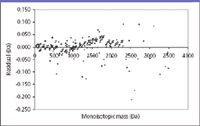
A second means through which an analyst can evaluate confidence in the regression analysis of data is a "residuals plot," which displays the deviation of the various measurement points from the regression value for an independent x value. As an example of this plot, and an example of quantitation in MS aside from the "How much?" question, Figure 2 (selected from Figure 7 in reference 4) presents mass error residuals found for a new mass adjustment method used in parallel post-source decay. Ideally, the deviations should occur on either size of the zero line. Clustering of the points would be a graphical indicator of systematic error that merits further investigation. The concentration of points adjacent to the zero line is evidence of a near-normal distribution, and the presence of the occasional point farther from the zero line heightens confidence in the method.

Figure 2: Residual plot for mass differences from the line of best fit for a mass calibration. The figure is from reference 4.

With a history of detailed evaluation and long application, an analyst might be inclined to assume that the underpinnings of linear regression analysis had been established. However, Renman and Jagner (5) used a computer simulation to show that a nonweighted linear regression analysis can produce results that are systematically overestimated if the calibration points are selected casually. These authors also delineate conditions in which the construction of a calibration curve using multiple standard additions can lead to less accurate results than if a single point calibration method is used. This conclusion is so at variance with standard accepted wisdom that even analytical textbooks sometimes falter in their clarity on this point. The conclusions of these authors show the practical consequences of previous work (6,7) revealing that results obtained when using standard addition calibration methods exhibit a non-Gaussian error distribution. When using the standard addition method, the magnitude of the addition itself affects the accuracy and precision of the analytical results (7). We often simplistically assume the opposite, so when confronted with the task of developing a standard analytical protocol for a targeted analyte within a constrained expected range of concentrations, a considered assessment of these factors should be primary. Additionally, when the protocol deviates from the expected conditions, due to exigencies of one sort or another, the likely deleterious effects on accuracy and precision must be taken into account.

In the next column, we discuss weighted linear regression and then provide a practical overview of the method of standard addition, again with discussion specific to application in MS. Then, in the final column of this series, we will attempt to show specific examples drawn from the recent published literature — both of extraordinary quantitation done well, and also perhaps some anonymous examples of results about which there might be some question. The latter selection is a particularly difficult task. In these examples, the overall conclusions might be justified, even though the supporting analytical results might be "almost but not quite right." In other venues, the conclusions ultimately might be found to be in error because the question originally posed was framed inadequately, rendering the uncertainty in the analytical results moot. In this series of columns, we have concentrated on the practical side of quantitative methods. If as a result, analysts become more confident of their understanding of quantitative practice, we will be better prepared to confront broader analytical issues, including the structuring of questions and the defense of results and attendant conclusions.

Kenneth L. Busch observes that his word processing program records the number of paragraphs, words, and characters in each "Mass Spectrometry Forum" column. The power of statistics is such that, with a sufficiently large sample of columns, an aggregate description of my writing style could be established, and the intervention of a ghostwriter might then be evident by a change in that metric. Such highly analytical work is not limited to the work of Shakespeare, or yours truly, but has current forensic uses. The material in this column represents opinions of the author and not those of the National Science Foundation. Contact the author at wyvernassoc@yahoo.com and send chocolate.

References

(1) H. Motulsky and A. Christopoulos, "Fitting Models to Biological Data using Linear and Nonlinear Regression: A Practical Guide to Curve Fitting," GraphPad Prism, Version 4.0. This is available as a printed publication, but is also available directly on line at www.graphpad.com/manuals/prism4/RegressionBook.pdf. Should you wish to print this file, the compilation is 351 pages in length.

(2) M.I. Ledvij, The Industrial Physicist 24–27 (April 2003). Available at www.originlab.com/index.aspx?s=9&pid=967.

(3) H. Motulsky, Intuitive Biostatistics (Oxford University Press, New York, 1995).

(4) D.J. Kenny, J.M. Brown, M.E. Palmer, M.F. Snel, and R.F. Bateman, J. Am. Soc. Mass Spectrom. 17, 60–66 (2006).

(5) L. Renman and D. Jagner, Anal. Chim. Acta 357, 157–166 (1997).

(6) K. Ratzlaff, Anal. Chem. 51, 232–235 (1979).

(7) M.J. Gardner and A.M. Gunn, Fresenius' J. Anal. Chem. 325, 263–266 (1986).