Raman Spectroscopy Analysis of Minerals Based on Feature Visualization

Raman spectroscopy is based on the Raman scattering effect discovered by the Indian scientist C.V. Raman. It analyzes the scattering spectrum with a frequency different from that of the incident light to obtain information about molecular vibration and rotation, and this information can be applied to the study of molecular structure.

Raman spectrometers have been proposed for the exploration of a diverse range of extraterrestrial targets including asteroids, Europa, Mars, the Moon, and Venus (1–8). The Mars Science Laboratory’s Chemistry and Mineralogy instrument (CheMin) analyzes the mineral content of rocks and sediments on Mars, including olivine and pyroxene, using X-ray diffraction (XRD) (9). Although this method has achieved good results, the collected samples need to be crushed during chemical analysis. The advantages of Raman spectroscopy, particularly its fast and nondestructive characteristics, can make it an effective alternative to XRD for such mineralogical analysis.

Given the weakness of the Raman signal, the original Raman spectrum obtained will generally contain obvious fluorescence background and noise, and various signal-processing procedures have been applied to extract useful information from the measured spectrum (10). Examples of such the signal-processing procedures include baseline correction, noise reduction, and statistical procedures, such as principal component analysis (PCA) and neural networks (11–15).

Balabin surveyed a number of machine-learning methods, including linear discriminate analysis (LDA), k-nearest neighbor, support vector machine (SVM), probabilistic neural networks (PNN), and multilayer perceptrons (MLP) as spectral classifiers for improving quality control in industrial gasoline production (16). Ryzhikova used serum near infrared (NIR) Raman spectroscopy combined with artificial neural network (ANN) classification models to diagnose Alzheimer’s disease (17). Data-driven deep learning approaches contribute to the discovery of intricate structures in high-dimensional data, reducing the need for prior knowledge and human efforts in feature engineering (18). Although the application of deep learning to Raman spectroscopy has improved performance, it is still difficult to intuitively understand the representations of this model.

Research into the visualization of deep learning not only helps to understand the working mechanism of the internal structure of the network, but also can help guide the research into neural networks in other applications, avoiding blind parameter adjustment or trials. Such research can also help users better understand deep learning models and make the results more powerful.

In the field of image classification, a visual explanation method for the convolutional neural networks (CNN) model has already been reported (19,20). The visualization of CNN-extracted features can help optimize the model. In this work, a lightweight network model for feature visualization in Raman spectrum analysis is proposed, termed factorization machine convolutional neural networks (FMCNN). While fully exploring the characteristics of the Raman spectral data of minerals, the results of analysis of the model are displayed transparently, and efficient and stable classification of the target samples are obtained.

Materials and Methods

Dataset Description

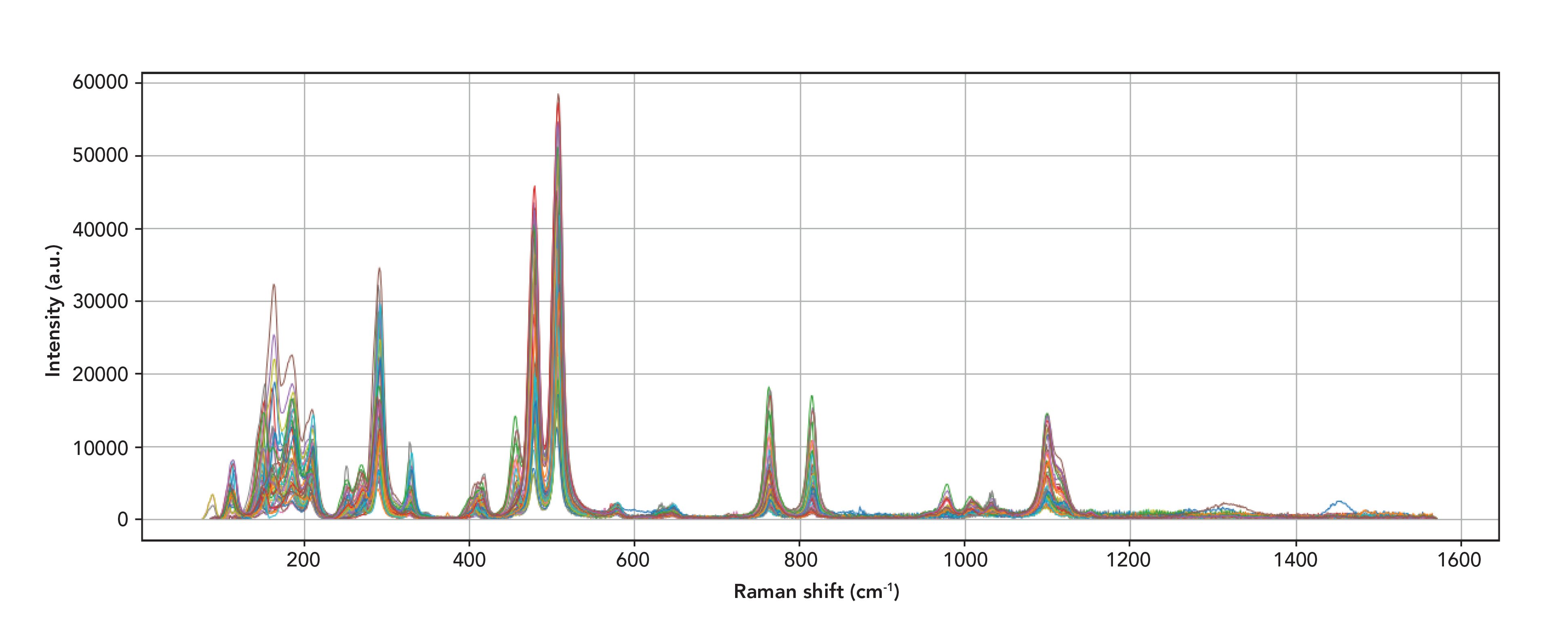
The RRUFF database was founded in 2006 at Arizona State University by Robert Downs. RRUFF currently contains tens of thousands of spectra acquired at several different laser wavelengths from oriented and un-oriented samples (21). For this project, we employed a subset of spectra from the RRUFF database, using only data from excellent oriented samples. This subset contains high-quality Raman spectral data for 222 minerals with a total of 3696 samples. After excluding spectra without independent mineral species identification from XRD analysis, and spectra containing only a single sample category, the number of categories dropped to 196, and the number of samples was 3284. Spectra for the mineral albite are shown in Figure 1, illustrating the typical within-class variance.

FIGURE 1: Raman spectra of Albite.

All samples have been baseline-corrected by the RRUFF project’s algorithm. Although there are several other methods for baseline correction, this study intentionally uses only standard RRUFF to process the data because most Raman communities use RRUFF data without modification. The Raman shift range of all the samples in this study is mostly between 0 and 1600 cm^-1. Given the different sources of spectrum collection, the samples have different sampling rates and measurement ranges. After comparing several different interpolation methods, we chose a simple linear interpolation method that aligns all features. Each spectrum is converted into a vector of 1360 intensity values and uniformly sampled at a common wavelength from 150 to 1510 cm^-1, making it convenient for further analysis.

FMCNN Model Architecture

This research proposes a lightweight network model, FMCNN, that is based on convolutional neural networks and is used to classify Raman spectral data of minerals. Figure 2 shows the detailed structure of the model. The network retains the input layer, a convolutional layer, a pooling layer, a flattening layer, a fully connected layer, and an output layer of the traditional CNN. At the same time, it introduces a batch normalization layer to enhance the generalization ability of the network and adds a fire-module to ensure that the width of the network is increased while minimizing the computational complexity (22). Given the local connection and shared weights, the modified model has fewer trainable parameters than a fully connected neural network.

FIGURE 2: FCNN model for Raman spectrum analysis.

First, the model receives preprocessed mineral Raman spectrum data. The input layer information is one-dimensional, and it contains the entire spectrum. Hence we train one-dimensional convolutional kernels in the model. For our convolutional layers, the activation function uses LeakyRelu to enhance the nonlinear fitting ability of the network, which is defined as:

where a is 0.2, which is TensorFlow’s initial parameter value (23). The convolutional layer is followed by a batch normalization layer (24).

The convolutional layer can be expressed as follows:

where X^xi is the i-th input map, Y^xj is the j-th output map, x is the wavenumber index of the input spectrum, w^ij denotes the weights of the convolution filter, * represents the convolution, and b^xj is a bias parameter of the j-th mapping. The function f indicates an activation function.

We introduced a fire-module after the first convolutional layer. This module specifically includes two parts, namely the squeeze layer and the expanded layer. The squeeze part is a convolution layer with a convolution kernel of 1 * 1, which is mainly used to reduce the number of input channels connected to this module, thereby greatly reducing the number of model parameters; the subsequent expanded part is composed of two convolution layers of size 1 * 1 and 3 * 3 (here our input is one-dimensional data, so 3 * 1 convolution layers are used instead of 3 * 3 convolution layers), which are mainly used for true feature maps. At the end of the module, a concatenate operation is performed to learn patterns from a limited number of variables. Increasing the depth of the network can extract low-level and high-level features from the original spectrum, and increasing the width of the network can improve the adaptability of the network to different scales of local spectral features.

The fire module is followed by a max-pooling layer for downsampling, and each neuron in the output map, Y, pools over a non-overlapping region in the input map, represented by X. Specifically,

The flattening layer connects the output of the fire module and converts it into a one-dimensional single vector, and then feeds it into the fully connected layer. The end of the model is to use the fully connected layers and followed by the softmax classifier to output the analysis results. The softmax function can be used to fit the input vector to real numbers in the range (in this case, the range is 0–1), and the sum of all real numbers is 1:

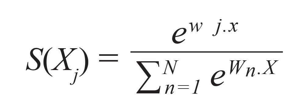
where X is an input vector, W_j is the weight of the j-th node, and N is the number of neurons in the output layer, which is the number of categories we need to test.

Visualization Method

The visualization method is based on the deconvolution network proposed by Zeiler (25). We reverse-mapped the middle layer features to the feature space. A deconvolution layer is attached to each layer of the fire module convolutional neural network (FMCNN). Deconvolution, also called transposed convolution, is the transposition of a conventional convolution layer filter. Figure 3 shows that convolution and deconvolution are two processes opposite to each other.

FIGURE 3: Illustration for (a) convolution verses (b) deconvolution.

Because the FMCNN model uses the max-pooling layer, only the largest features are retained when extracting features, and non-maximum feature information is lost. In the process of forwarding calculation of maximum pooling, we use a table to record the position of each maximum value. When unpooling the feature, the maximum value is marked back to the recorded position, and zeros are filled in where the rest of the information is lost.

For the activation function in the model, we use LeakyRelu to increase the non-linear relationship between the network layers. Similarly, in the deconvolution process, the reconstructed signal obtained from the previous layer is sent to the LeakyRelu function for calculation, and high-level semantic information in the data is mined.

This research only visualizes the features in the convolutional layers so after the network training is completed, the flatten layers and softmax layers in the model can be ignored. Using the transpose of the trained convolution kernel to convolve the output features of each layer of the neural network, we can get the visualization results.

Model Training

While training the network, we use classification cross-entropy error loss and L2 norm regularization to minimize the sum of squares and prevent overfitting:

where m is the number of categories of observation samples, n is the number of samples in the training set, h(X_ji) and Y_ji are measured values and predicted values, W is the weight matrix, and λ is the regularization coefficient.

We used an Adam optimizer for parameter learning, which can iteratively update neural network weights based on training data (26). The learning rate is equal to 0.001 (lr = 0.001), the exponential decay rate of the first moment estimate is 0.9 (beta_1 = 0.9), the exponential decay rate of the second moment estimate is 0.999 (beta_2 = 0.999), and epsilon is 1e-08. An early stopping strategy is deployed to prevent overfitting.

Comparison with Other Methods

To compare the FMCNN model with conventional analysis approaches, we consider a number of alternative machine-learning methods: KNN, RandomForests (RF), SVM, and LDA.

Parameters of all the models have been optimized toward improved model performance. For the KNN model, the grid search method was used for parameter optimization, and the optimal value of the parameter K was determined (k = 1). For the RF model, we built 500 sub-trees to make the model have better prediction results. SVM is a kernel-based machine learning algorithm. In this experiment, the linear kernel function (penalty factor C = 100, gamma = 0.0078) was selected after comparison. All the models are implemented on the Python platform using Keras and Scikit-learn library.

Evaluation Protocol

Validation is a crucial step in developing classification models because neural networks can frequently be overtrained (17). Because there are usually only a handful of spectra available for each mineral, the feasibility and effectiveness of the model were evaluated using a 10 times 10-fold cross-validation method. Specifically, the dataset is divided into ten parts, one of which is used as test data in turn, and the remaining nine are used as training data. The whole process was repeated ten times, and the average of the 10 results was used as an estimate of the algorithm’s accuracy.

Results

Table I shows a comparison of the results of the FMCNN model performance and those of other traditional machine learning analysis methods. Table I also shows the mean and standard deviation of the accuracy of the 10 times 10-fold cross-validation for all the methods. The results show that in each of the results of all models, the FMCNN model obtained the best results, with an average prediction accuracy of 0.988. Compared with the worst-performing LDA, the average accuracy is improved by 15%. Compared to the best performing SVM, the average improvement is 2.4%.

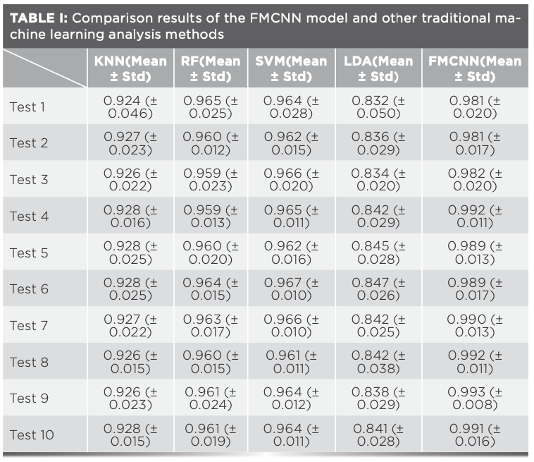
Figure 4 shows a comparison of the classification stationary results of ten experiments of all the methods. After all methods were optimized, 10-fold cross-validation was carried out ten times. Although the waveforms have some fluctuations, the amplitude is not large. The accuracy of the FMCNN model proposed in this paper is significantly higher than that of all other methods. The waveform is smooth and the model has strong stability, which indicates that the model has good application potential in Raman spectrum analysis of minerals.

FIGURE 4: Mean accuracy comparison results for all classification methods (stationary).

For a deep learning network model, after multiple convolutions and pooling, the middle layer contained rich spatial and semantic information. The final flattening layer and the fully connected layer will lose the spatial information of the input data. It is difficult to show this visually. Therefore, to reasonably explain the classification results of the FMCNN model, it is necessary to make full use of the pooling layer before the flattening layer.

Figure 5 shows part of the test mineral spectrum used for evaluation and the visualization results of the characteristics of the pooling layer extracted by this spectrum. The first line shows part of the evaluation spectrum used for the test, and the second line corresponds to the features extracted from the test spectrum. It can be seen in Figure 5 that the extracted features include strong Raman peaks corresponding to the mineral spectrum. In the FMCNN model, the extracted features can indicate the weights used to classify the test data set. Specifically, if a mineral spectrum has a strong Raman peak at a certain region, and the strong peak does not appear in another mineral spectrum, then the activation value of the feature map represented by this strong peak is large in the forward propagation process. In contrast, if there is a similar strong peak in the vicinity of the strong peak in another mineral spectrum, the activation value of the feature map of the strong peak will be small. Therefore, the extracted feature visualization results in the second row of Figure 5 corresponding to the shape of the test spectrum in the first row. The extracted features had strong highlights at strong Raman-peak regions, and near-zero values were obtained at the background level region.

FIGURE 5: Top row shows different Raman mineral spectra, namely (a) actinolite, (b) adamite, (c) witherite, and (d) zircon. Bottom row shows corresponding Raman extracted spectral features contributing to the recognition for each mineral (e) actinolite, (f) adamite, (g) witherite, and (h) zircon, respectively. The x-axis label for the top row spectra is Raman shift (cm-1) and for the bottom row features it is Wavenumbers (cm-1). The y-axis label for the top row spectra is Intensity (a.u.) and for the bottom row features Intensity.

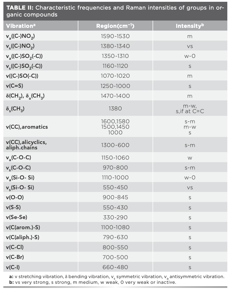
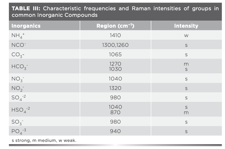
Raman spectroscopy can reflect the molecular structure and conformation information, and this information is the key basis for minerals to be accurately distinguished. Table II shows some characteristic bands, including the characteristic frequency and Raman intensity of groups in organic compounds (27). Table III shows the characteristic frequencies and Raman intensity of groups in some common inorganic compounds (28). The special chemical and structural differences between various types of minerals can be reflected in the corresponding information on the Raman spectrum. These characteristics are analyzed using deep learning methods, and finally, the classification can be accurately completed.

Conclusion

We have proposed a lightweight network model for the feature visualization of Raman spectroscopy analysis, called the FMCNN model. The study discussed in this article proved that the method is simple in structure and easy to implement. Compared to other well-known machine learning methods, the accuracy of the model was higher while the stability of the model is guaranteed. It has a broad application prospect for the analysis of mineral Raman spectra.

The ability of the model to interpret mineral Raman spectra is essential for the further development of spectral analysis using deep learning methods. The application of a feature visualization method, which reversely maps the features of the middle layer to the pixel space, is important for the advancement of Raman spectroscopy. Therefore, the model can be visualized to analyze the process of neural network feature extraction.

This process can help identify key Raman bands related to feature analysis. The evaluation of the experimental results also confirms the accuracy of the feature extraction method. The method can be used to validate trained models to ensure the reliability of the classification of multiple mineral samples.

Finally, considering the characteristics of the spectral data, we also considered applying this method to other types of spectral and other material analysis. We speculated that this can be effectively achieved by fine-tuning the model.

References

(1) W.G. Kong, and A. Wang, “Planetary laser Raman spectroscopy for surface exploration on C/D-type asteroids—a case study,” paper presented at the Lunar and Planetary Science Conference, Lunar and Planetary Institute, Houston, Texas, 2010.

(2) S. Michael Angel, R.G Nathaniel, K.S. Shiv, and M.K. Chris, Appl. Spectros. 66, 137–150 (2012). https://doi.org/ 10.1366/11-06535

(3) P. Sobron, C. Lefebvre, A. Koujelev, and A. Wang, “Why Raman and LIBS for Exploring Icy Moons?” paper presented at the Lunar and Planetary Institute Science Conference, Lunar and Planetary Institute, Houston, Texas, 2013.

(4) S.K. Sharma, and P.G. Lucey, Spectrochim. Acta. A. 59, 2391–2407 (2003). https://doi.org/ 10.1016/j.saa.2013.06.053

(5) A. Wang, L.A. Haskin, A.L. Lane, T.J. Wdowiak, S.W. Squyres, R.J. Wilson, L.E. Hovland, K.S. Manatt, N. Raouf, and C.D. Smith, J. Geophys. Res. 108, 1991–2012 (2003).

(6) P. Sobron, F. Sobron, A. Sanz, and F. Rull, Appl. Spectros. 62, 364–370 (2008).

(7) Z.C. Ling, A. Wang, B.L. Jolliff, C. Li, J. Liu, W. Bian, X. Ren, and Y. Su, “Raman spectroscopic study of quartz in lunar soils from Apollo 14 and 15 missions,” paper presented at the Lunar and Planetary Science Conference, Houston, Texas, 2009.

(8) J.L. Lambert, J. Morookian, T. Roberts, J. Polk, S. Smrekar, S. M. Clegg, R.C. Weins, M.D. Dyar, and A. Treiman, “Standoff LIBS and Raman spectroscopy under Venus conditions,” paper presented at the Lunar and Planetary Science Conference, Houston, Texas, 2010.

(9) D. Blake, “The development of the CheMin XRD/XRF: reflections on building a spacecraft instrument,” paper presented at the IEEE Aerospace Conference, Big Sky, Montana, 2012.

(10) T. Bocklitz, A. Walter, K. Hartmann, P. Rosch, and J. Popp, Anal. Chim. Acta. 704, 47–56 (2011). https://doi.org/10.1016/j.aca.2011.06.043

(11) N.K. Afseth, V.H. Segtnan, and J.P. Wold, Appl. Spectrosc. 60, 1358–1367 (2006). https://doi.org/10.1366/000370206779321454

(12) G. Schulze, A. Jirasek, M. Yu, A. Lim, R. Turner, and M. Blades, Appl. Spectrosc. 59, 545–574 (2005). https://doi.org/10.1366/0003702053945985

(13) P.J. Grood, G.J. Postma, W.J. Melssen, L.M.C. Buydens, V. Deckert, and R. Zenobi, Anal. Chim. Acta. 446, 71–83 (2001). https://doi.org/ 10.1016/S0003-2670(01)01267-3

(14) S. Sigurdsson, P. Philipsen, L. Hansen, J. Larsen, M. Gniadecka, and H. Wulf, IEEE Trans. Biomed. Eng. 10, 1784–1793 (2004). https://doi.org/10.1109/tbme.2004.831538

(15) S. Feng, D. Lin, J. Lin, B. Li, Z. Huang, G. Chen, W. Zhang, L. Wang, J. Pan, R. Chen, and H. Zeng, Analyst 138, 3967–3974 (2013). https://doi.org/10.1039/C3AN36890D

(16) R.M. Balabin, R.Z. Safieva, and E.I. Lomakina, Analytica Chimica Acta. 671(1–2), 27–35 (2010). https://doi.org/10.1016/j.aca.2010.05.013

(17) E. Ryzhikova, O. Kazakov, and L. Halamkova, J. Biophotonics 8(7): 584–596 (2015). https://doi.org/10.1002/jbio.201400060

(18) Y. LeCun, Y. Bengio, and G. Hinton, Nature 521, 436–444 (2015). https://doi.org/10.1038/nature14539

(19) D. Smilkov, N. Thorat, B. Kim, F. Viegas, and M. Wattenberg, “Interpretability Beyond Feature Attribution: Quantitative Testing with Concept Activation Vectors (TCAV),” paper presented at the International Conference of Machine Learning in Sydney, Australia, 2017.

(20) R.R. Selvaraju, M. Cogswell, A. Das, R. Vedantam, D. Parikh, and D. Batra, “Quantitative Phase Imaging and Artificial Intelligence: A Review,” paper presented at International Conference of Machine Learning in Sydney, Australia, 2017.

(21) R.T. Downs, “The RRUFF Project: an integrated study of the chemistry, crystallography, Raman and infrared spectroscopy of minerals,” paper presented at the Program and Abstracts of the 19th General Meeting of the International Mineralogical Association in Kobe, Japan, 2006.

(22) F.N. Iandola, S. Han, and M.W. Moskewicz, K. Ashraf, W.J. Dally, and K. Keutzer, “Squeezenet: Alexnet-level Accuracy With 50X Fewer Parameters and <0.5MB Model Size,“ paper presented at the International Conference on Learning Representations, Toulon, France, 2017.

(23) A.L. Maas, A.Y. Hannun, and A.Y. Ng, “Rectifier nonlinearities improve neural network acoustic models,” paper presented at the ICML Workshop on Deep Learning for Audio, Speech and Language Processing, Atlanta, Georgia, 2013.

(24) S. Ioffe and C. Szegedy, “Batch normalization: accelerating deep network training by reducing internal covariate shift,” paper presented at the International Conference on Machine Learning, Miami, Florida, 2015.

(25) M.D. Zeiler, D. Krishnan, and G.W. Taylor, “Deconvolutional networks,” paper presented at the IEEE Conference on Computer Vision and Pattern Recognition, San Francisco, California, 2010.

(26) D. Kingma and J. Ba, “Adam: A Method For Stochastic Optimization,” paper presented at the International Conference of Learning Representations, San Diego, California, 2015.

(27) I.B. Schrader, Angew. Chem. Int. Ed. Engl. 12(11): 884–908 (1973). https://doi.org/10.1002/anie.197308841

(28) P. Larkin, in Infrared & Raman Spectroscopy (Elsevier, Waltham, Massachusetts, 2nd ed., 2018), pp. 85–134.

Zhiqi Guo, Shengwei Tian, Xiaoyi Lv, and Wenlong Xue are with the College of Software at Xinjiang University, in Urumqi, China. Long Yu is with the College of Network Centers at Xinjiang University, in Urumqi, China. Direct correspondence to Long Yu at yul_xju@163.com.