Simultaneous Detection of Nitrate and Nitrite Based on UV Absorption Spectroscopy and Machine Learning

Using spectrophotometry to acquire nitrate and nitrite concentrations is common in water quality monitoring. However, it is challenging to achieve the measurement with high accuracy because of the spectral signal overlapping. In this article, a hybrid machine learning approach is proposed to simultaneously determine nitrate and nitrite based on UV absorption spectroscopy. All spectral data are divided into four subdivisions according to the concentration ratio of nitrate and nitrite. In each subdivision, a regression submodel is established according to the sample characteristics. First, the sample is voted to a category by a joint classifier and then processed by the corresponding submodel to predict the concentrations of nitrate and nitrite. This method has been further optimized by considering the interference of foreign ions. The proposed approach improves the performance of spectral direct detection and is therefore a promising tool for fast determination and continuous monitoring in environmental applications.

Nitrate (NO₃ ̄) and nitrite (NO₂^-) are the most common forms of nitrogen that are found in environments, physiological systems, and food industries (1,2). Excessive nitrate and nitrite lead to the eutrophication of an ecosystem, which introduces fatal threats to human health, such as methemoglobin syndrome (3). Considering their pollution hazards, regulations have been imposed to set legal limits of nitrate and nitrite in water worldwide. Therefore, it is critical to find convenient and economical methods to monitor these trace analytes. A broad range of techniques have been evaluated to monitor nitrate and nitrite in water, including electrochemical detection, chemiluminescence, colorimetric analysis, and UV spectrophotometry (4–7). Among various approaches, direct UV absorption spectrophotometry has attracted attention in the past decades for its high speed, reagent-free, operational simplicity, and ultralow cost operation (8–10).

The absorption spectra of nitrate and nitrite are similar and nearly overlap in the UV region (11). Hence, it is difficult to separate nitrate and nitrite contributions from the collected spectra. Wetters and Uglum first proposed to use the secondary peak of the absorption spectra to detect nitrate and nitrite at high concentrations (12). After that, Suzuki and Kuroda used the isosbestic absorption points of the second derivative spectra for determining nitrate and nitrite simultaneously (13). Both methods were based on the intrinsic absorption properties of nitrate and nitrite at two special wavelengths, and the models would be greatly affected by the interfering substances. To increase the accuracy, several methods that employed multiple wavelengths were proposed to achieve simultaneous measurements of nitrate and nitrite. Dong and others used a matrix algorithm to select six points in a narrow wavelength interval (14). Rieger and others adopted a multivariate correction algorithm with a total of 256 wavelengths uniformly spaced in the range of 210–400 nm (15). Sandford and others established the reference spectra of nitrate, nitrite, and bromide to achieve the simultaneous measurement based on the deconvolution method (16). However, these approaches for choosing an optimal modeling range are too approximate and inevitably some useful spectral information is lost. In addition, environmental noise, experimental error, and redundant information with low information content is contained in the spectral data. All such factors reduce the stability and accuracy of the measurement.

Machine learning methods offer versatile and powerful solutions in spectra analysis, such as characteristic extraction, component classification, and concentration prediction (17–19). Recently, the combination of UV spectroscopy and machine learning has been successfully applied in the rapid detection of multiple compounds (20–22). However, most of the machine learning methods are based on a single model, which has prominent limitations in optimizing evaluation accuracy. Hence, some researchers have tried to build a hybrid model based on clustering algorithms to predict certain water quality parameters (23). The hybrid model has demonstrated a higher prediction accuracy than a single model.

In this work, a hybrid machine learning model is developed for direct measurement of nitrate and nitrite based on UV absorption spectroscopy. First, a joint classifier (JC) is utilized to divide the samples into four subregions based on the concentration ratios between nitrate and nitrite. Then, a submodel is selected for regression prediction in each subregion. To the best of our knowledge, this model is the first demonstration of simultaneous detection of nitrate and nitrite using a hybrid machine learning model combining classification and regression algorithms. Compared to other direct spectral methods, the proposed method with the advantages of machine learning can more effectively use the spectral information of the samples, enhancing the sensitivity of detection, especially for extremely low concentrations. For example, the average relative errors in determining nitrate and nitrite are approximately 4–5% by using the second derivative spectroscopy (13) and matrix method (14). The proposed machine learning method reduces the average relative errors to a value below 1%. In addition, the interference effects of wavelength selection and foreign ions on this method has been discussed.

Theory and Methods

Classification

Support vector machines (SVM) are multiclassifiers based on the statistical learning theory (24). The basic model of SVM is defined as the linear classifier with the largest interval in the feature space. In this work, the spectral data are normalized before being processed by SVM because the convergence of the training network can be accelerated by mapping the data to a range of 0~1. Because abundant data increase the quantity of computation, principal component analysis (PCA) (25), which can eliminate multicollinearity existed among variables, is used to reduce the data dimension of the input layer. The particle swarm algorithm (PSO) (26) optimizes the penalty factor and kernel parameters in the modeling process. The overall program is built on the Libsvm toolbox (27,28).

Logistic regression (LR) is an algorithm that assumes data obey a binomial distribution and applies the maximum likelihood function to achieve binary classification of samples (29). When the samples are going to be divided into multiple categories, LR is employed to build an independent binary classifier for each category.

Random forest (RF) is another algorithm for classification (30). It consists of multiple decision trees, in which the training samples are obtained by bootstrap sampling from the original training set. In addition, RF utilizes random feature selection in the growth process of the decision tree, which prevents overfitting. For classification, an unknown sample is sent to each decision tree for prediction, and then voted for classification. The class with the most votes is the final classification result.

The above three classifiers are used as the base classifiers to vote for the categories of the same sample, which can effectively improve the reliability and robustness of the system.

Feature Selection

Modeling with all wavelength points increases model complexity and reduces accuracy because of the huge amount of data and redundant information in the full-range spectrum. Each wavelength point is different in terms of the amount of useful information and the degree of interference by other ions. Therefore, it is necessary to screen out useful variables with high sensitivity and correlation to the target ions, while eliminating redundant variables sensitive to foreign ions. In this work, stability and variable permutation (SVP) is used to choose the characteristic wavelengths. Variables are selected through multiple iterations and competitions in SVP (31). After all iterations are completed, model population analysis is employed to obtain the optimal subset of variables with the minimum mean and relatively low standard deviation value of root mean square error.

Regression Model

A regression model is used to establish the relationship between input variables and output variables. As the most commonly used regression algorithm in spectral multivariate correction analysis, partial least square (PLS) is a perfect combination of multivariate linear regression, canonical correlation analysis, and PCA (32). As an alternative regression algorithm, least squares support vector machine (LSSVM) is an improved version of the SVM algorithm. It uses the least squares linear system as the loss function, and reduces the computational complexity by solving a set of linear equations instead of the more complex quadratic programming method used by the traditional SVM (33).

Experiments

All reagents were of analytical grade (Sinopharm Chemical Reagent Co., Ltd) and used without further purification. Nitrate and nitrite stock solutions (100 mg N/L) were prepared by dissolving 0.7221 g of potassium nitrate and 0.4928 g of sodium nitrite in 1 L of deionized water, respectively. A series of measurements were made for nitrate and nitrite solutions with 10 different concentrations, ranging from 0.1 to 3.0 mg N/L. A total of 100 groups of mixture solutions were investigated and used as training data in the machine learning models. Instead of dividing the samples into calibration and validation sets, leave-one-out cross validation (34) was used as an evaluation strategy. These solutions were prepared by serial dilution in deionized water from the nitrate:nitrite stock solution. Sodium chloride, sodium bromide, sodium carbonate, sodium bicarbonate, calcium chloride, magnesium chloride, and humic acid were added in the mixture solutions for the interference studies.

UV spectra were acquired with a dual beam UV-vis spectrophotometer (UV-2600, Shimadzu). Deionized water was used as a reference solution. Samples were scanned between 190 and 400 nm in a quartz cuvette with a 10-mm optical pathlength. Scans were conducted at 120 nm/min with a resolution of 1 nm. Each measurement was repeated three times to ensure reproducibility.

Results and Discussion

Division Based on Concentration

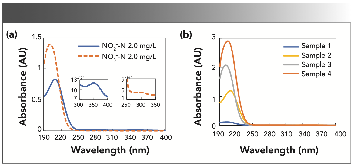
Figure 1a shows the UV spectra of nitrate and nitrite solutions, which both have a wide absorption peak between 190–250 nm, thus several methods for the measurement of nitrate and nitrite concentrations depend on the absorbance at wavelengths approximately at 200 nm (12–14,16). In fact, there is a second absorption peak for nitrate and nitrite above 250 nm, as shown in the insets of Figure 1a. Because the second absorption peak is relatively weak and has a small value, the spectrum above 250 nm in Figure 1a was flattened by the high absorbance for the region below 250 nm. However, this spectral region may still contain useful information for modeling. Figure 1b shows the spectral curves of four mixture samples with different concentrations. The absorbance difference between the mixtures of nitrate and nitrite with the maximum and minimum concentrations is nearly 40 times. In a preliminary study, we analyzed the spectral data with centralized modeling, in which the mixture solutions with different concentrations were calculated by the same model. It has been found that centralized modeling has insufficient sensitivity to predict components at low concentrations because of the wide modeling range of samples.

FIGURE 1: The original spectra of the samples. (a) UV absorption spectra of pure nitrite and nitrate solutions with the concentration of 2 mg N/L (Note that nitrate-N (mg/L) = 0.2259 x nitrate-NO₃ (mg/L), and nitrite-N (mg/L) = 0.3044 x nitrite-NO₂ (mg/L)). The insets show the second peaks of nitrite and nitrate, respectively. (b) UV absorption spectra of mixture samples. Sample 1: 0.1 mg N/L nitrate and 0.1 mg N/L nitrite; sample 2: 0.1 mg N/L nitrate and 3 mg N/L nitrite; sample 3: 3 mg N/L nitrate and 0.1 mg N/L nitrite; and sample 4: 3 mg N/L nitrate and 3 mg N/L nitrite.

To achieve a more accurate prediction, the concentrations of nitrate and nitrite are divided into four subregions for separate modeling. Each subregion has its own distinct characteristics related to the concentration ratio between nitrate and nitrite. In region 1, the concentrations of nitrate and nitrite are both low; in region 2, the nitrite concentration is much higher than that of nitrate; in region 3, the nitrite concentration is much lower than that of nitrate; and in region 4, the concentrations of nitrate and nitrite are both high. In this way, each submodel has higher prediction accuracy than centralized modeling as it adapts to the sample characteristics of each region.

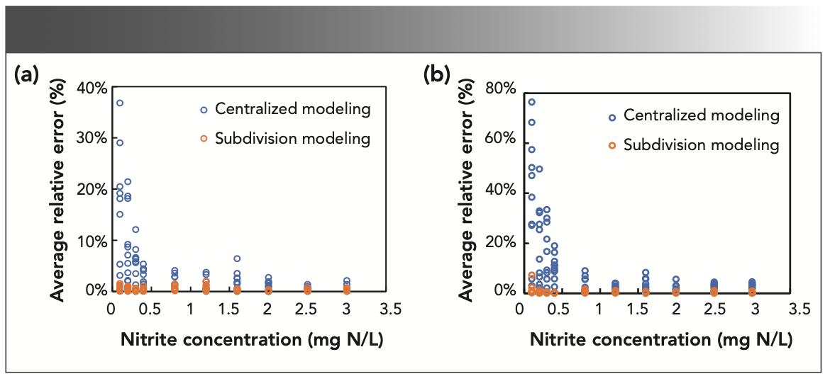
We performed modeling analysis on 100 experimental samples, and com- pared the performance of centralized modeling and division modeling in predicting the concentrations of nitrate and nitrite. The results are shown in Figure 2. Although the average relative errors in centralized modeling are small (<10%) with relative high concentration of analytes, it greatly increases when the concentration is lower than 0.4 mg N/L. By contrast, the division modeling always gives a stable and satisfied performance with an average relative error less than 5%. In view of the insufficient predictive sensitivity at low concentrations, the critical concentration used to divide subregions is chosen to be placed at a lower position. We compared the modeling results, which set the critical concentrations as 0.3, 0.4, and 0.8 mg N/L, respectively. The division modeling gives a highest accuracy (~98%) and lowest average relative errors (~0.44%), when the critical concentration is 0.4 mg N/L. Therefore, the critical concentration is set to 0.4 mg N/L for the following modeling procedures.

FIGURE 2: Comparison of the average relative errors of centralized modeling and division modeling in determining (a) nitrate and (b) nitrite. The critical concentration used for division modeling was 0.4 mg N/L. Only support vector machines (SVM) was used for classification here.

Classification

The overall program framework is shown in Figure 3. First, the collected spectral data are classified by three classifiers (SVM, LR, and RF) independently. Based on voting results, the data are sent to the submodels or analyzed by the centralized modeling. In each model, SVP is used to select characteristic wavelength, and PLS is utilized to build the regression model. Finally, the predicted concentrations of nitrate and nitrite are given out simultaneously.

FIGURE 3: Flow chart of the machine learning program framework.

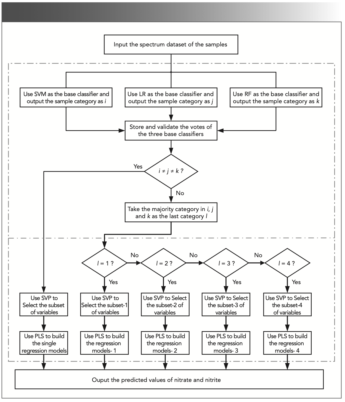
Because the program is executed sequentially, and to avoid the classification error from affecting the subsequent regression accuracy later, a joint classifier composed of SVM, LR, and RF is used to vote on the sample category. The sample is classified into the category with the majority of votes (≥2). If the categories selected by the three classifiers are all different, the classification result is determined to be unreliable and a corresponding reminder is given. In this case, a single non-classified regression model is used for prediction, so that the accuracy can be at least consistent with that of centralized modeling. It is worth mentioning that each submodel is built with samples distributed on the classification boundary to avoid larger prediction errors caused by classification errors. Because the probability of classifiers making errors at these points are greater. In the experiments, the classification accuracy using RF, LR, and SVM reached 94%, 97%, and 98%, respectively. There were 11 samples that were misclassified by the three base classifiers among the 100 experimental samples. Three samples were actually located on the classification boundary, so their influence on the prediction results can be ignored. In addition, other samples that were misclassified in a single classifier finally got the right classification results because of the voting mechanism. The fault tolerance and robustness of the system are greatly improved because of the joint classifier.

Wavelength Selection

The optimal wavelength set is supposed to combine the specific characteristics of nitrate or nitrite. For each subregion, SVP selects only one subset of variables (that is wavelength) for nitrate and nitrite, respectively. Parameters in SVP are optimized using grid search. The model using the specialized subset of variables can achieve better performance because it adapts to the characteristics of the target ions in a narrow concentration range. The numbers of optimal variables are different in the submodels, which are changing from eight to 34. The number is related to the spectral similarity of the samples in each subregion. The regression models are built based on these variables.

Performance Evaluation

Four classical parameters were employed to evaluate the performances of the established models, including average relative error (ARE), maximum relative error (MRE), root mean square error of prediction (RMSEP), and determination coefficient (R²). The RMSEP is expressed as:

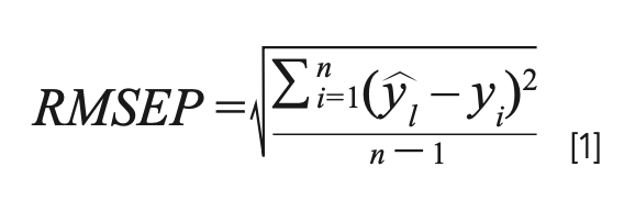
where n is the total number of samples, ŷ_i is the actual value of sample i, and ŷ_i is the predicted value of sample i. The determination coefficient (R²) is expressed as:

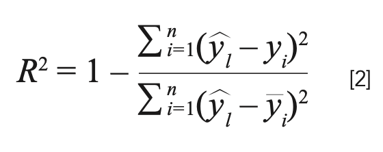
where ŷ_i is the average value of all the testing samples. According to equations 1 and 2, the model performs better with lower RMSEP and higher R².

The performances of different algorithms are compared in Table I. The centralized modeling only builds a single model, in which SVP and PLS are used for wavelength selection and regression modeling, respectively. Division modeling 1 uses the joint classifier for classification, followed by submodeling with SVP and PLS. Division modeling 2 also employs joint classifier. Then, the Savitzky-Golay method (35) is used to obtain the second derivative of the original spectral data, which are subsequently processed by SVP. Finally, the regression model is established using LSSVM. To enhance the generalization ability of the model in the entire concentration range, the centralized modeling inevitably sacrifices the local accuracy, which has much greater error values as shown in Table I. Compared with it, division modeling 1 uses the same feature selection and modeling methods, but only employs the joint classifier to classify the samples in advance. This method improves the accuracy of prediction significantly, especially for low concentration samples. When the centralized modeling is replaced by division modeling 1, the average relative error is reduced from 4.16 to 0.44% for nitrate, and from 10.26 to 0.54% for nitrite. The maximum relative error of nitrate has even decreased 18 times. It proves that division modeling has the potential to expand the modeling range without reducing the prediction accuracy. Division modeling 2 employs the differential preprocessing to expand the distance between the spectral peaks of nitrate and nitrite that are almost overlapped. However, the results show that the effect is not significant, because the spectra of the two analytes in the 200–250 nm range are approximately parallel, which yields the same information trends using the same pre- treatment. The maximum relative error of division modeling 2 is close to four times that of division modeling 1 in the prediction of nitrate. It is because most of the spectral signals still have linear additivity in a two-component experimental system with relatively simple spectra. It is consistent with the modeling scenario of PLS, which is a multiple correction method based on linear regression. In contrast, LSSVM is a nonlinear correction method. In addition, PLS can also overcome the interference of nonlinear factors to a certain extent, bringing advantages in spectral multivariate correction analysis.

Influence of Foreign Ions

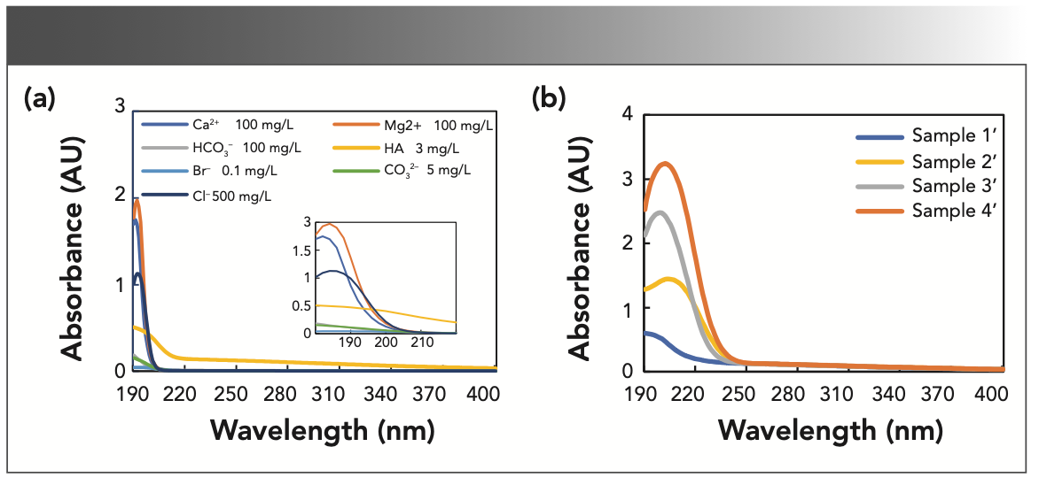
In actual water samples, there are many other ions that also absorb UV light, which probably affect the measurement of nitrate and nitrite (14,36,37). The influence of several common ions in water has been investigated. The individual spectra of these substances are shown in Figure 4a. It can be seen that most of the foreign ions only have absorption at 190–205 nm, whereas humic acid (HA) representing organic matters has an absorption band after 205 nm that is not negligible.

FIGURE 4: (a) UV absorption spectra of foreign ions. (b) The spectra of four samples from different regions affected by HA (3 mg/L). Sample 1’: 0.1 mg N/L nitrate and 0.1 mg N/L nitrite; sample 2’: 0.1 mg N/L nitrate and 3 mg N/L nitrite; sample 3’: 3 mg N/L nitrate and 0.1 mg N/L nitrite; and sample 4’: 3 mg N/L nitrate and 3 mg N/L nitrite.

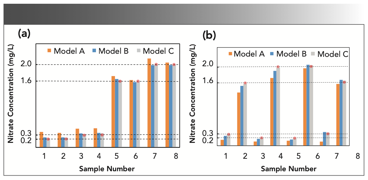
Wavelength selection plays an important role in reducing the influence of foreign ions. For instance, 500 mg/L chloride ion was added into eight groups of nitrate and nitrite mixtures with four concentration levels (0.2, 0.3, 1.6, and 2 mg N/L). The concentrations of the eight samples are symmetrically distributed in four subregions. We compared the performance of three models with different modeling methods. Model A uses 200 nm as the starting wavelength for centralized modeling. Model B and Model C use 200 nm and 205 nm as the starting wavelengths for division modeling, respectively. The final prediction results are shown in Figure 5. It can be seen that the predicted concentrations using model A are far from the true values. The relative errors are even more than 50% for low concentration samples (<0.4 mg N/L). On the contrary, Models B and C are much closer to the true values, which verifies the improvement by using the division modeling method. The average relative errors are 18% and 6% in Models B and C, respectively. It means that the chloride ions have little influence on the prediction of nitrate and nitrite, when the starting wavelength of modeling is delayed to 205 nm.

FIGURE 5: Test results of different models when chloride ions are added in the mixture samples. The determination targets are (a) nitrate and (b) nitrite, respectively. A red ball marker passing through the dash line above each sample is used to highlight the true concentration of the analyte.

The concentrations of nitrate and nitrite mixtures were measured with various interfering ions as shown in Table II. Concentration of a foreign ion was chosen when its absorbance equaled 0.1 approximately at 205 nm. Each type of foreign ions was added to the eight groups of nitrate and nitrite mixtures. Table II shows the influence of these foreign ions on the prediction results of Model C. The joint classifier still worked well in the presence of foreign ions, except for HA. Misclassification occurs when samples are assigned to a different category than the one they should be in. For example, a sample in region 1 is assigned to region 2. The experimental results showed that one sample was misclassified after adding Ca²⁺, Mg²⁺, CO₃^2-, and HCO₃^-. It is worth noting that the misclassified samples are all in region 3 with the same concentrations of nitrate (1.6 mg N/L) and nitrite (0.2 mg N/L). A possible explanation comes from the concentration ratio of nitrate to nitrite in this sample, which is the highest among the eight samples. The absorption spectra of nitrate and nitrite are almost overlapped. When the concentration ratio of nitrate to nitrite is increased, it is more difficult to identify the contribution from nitrite in the spectra of mixture samples. Because the proportion of nitrate and nitrite in the total absorbance is a potential internal consideration in the model, the classifier may be affected by the concentration ratio. For the same reason, the relative error in the determination of nitrite is often higher than that of nitrate.

The average relative error caused by the interference of foreign ions mostly can be controlled within 10%. Because of the wide absorption band of HA in the range of 205–400 nm, after adding HA to the mixture, the absorbance of the sample in this spectral range will increase as shown in Figure 4b. In addition, the increase at each wavelength point may not be the same. This change causes the classifier to make wrong judgments on the concentration of nitrate and nitrite, resulting in misclassification and further large prediction errors. Thus, all eight representative samples have a high possibility to be misclassified. Therefore, incorporating the organic ions into the modeling components when there are more organic interferences in the water samples is recommended.

Conclusion

To summarize, we proposed a hybrid machine learning method to tackle the challenge of predicting nitrate and nitrite simultaneously with UV absorption spectroscopy. Compared with centralized modeling in other spectroscopic methods, the proposed model provides higher accuracy by employing a joint classifier before the regression modeling. The influence of classification, wavelength selection, and foreign ions are discussed to optimize the model. This method is fast, reagent-free, and potentially useful for developing in situ sensors for monitoring trace species in marine and aquatic environments. In addition, the proposed methodology can also be applied to determine multiple composite substances. The proposed methodology holds broad application prospects in water quality monitoring, food safety, and soil properties qualification.

Funding

This work was supported by the State Key Program of the National Natural Science Foundation of China (Grant No. 61890932).

References

(1) M.J. Moorcroft, J. Davis, and R.G. Compton, Talanta 54, 785–803 (2001).

(2) Q.H. Wang, L.J. Yu, Y. Liu, L. Lin, R.G. Lu, J.P. Zhu, L. He, and Z.L. Lua, Talanta 165, 709–720 (2017).

(3) A.M. Fan, C.C. Willhite, and S.A. Book, Regul. Toxicol. Pharm. 7, 138–148 (1987).

(4) P. Singh, M.K. Singh, Y.R. Beg, and G.R. Nishad, Talanta 191, 364–381 (2019).

(5) M. J. Moorcroft, L. Nei, and J. Davis, Anal. Lett. 33, 3127–3137 (2000).

(6) T. Aokia, S. Fukuda, Y. Hosoi, and H. Mukai, Anal. Chim. Acta 349, 11–16 (1997).

(7) R.B.R. Mesquita, M.T.S.O.B. Ferreira, R.L.A. Segundo, C.F.C.P. Teixeira, A.A. Bordalo, and A.O.S.S. Rangel, Anal. Methods 1, 195–202 (2009).

(8) H.E. Khorassani, P. Trebuchon, H. Bitar, and O. Thomas, Water Sci. Technol. 39, 77–82 (1999).

(9) R.S. Brito, H.M. Pinheiro, F. Ferreira, J.S. Matos, and N.D. Lourenco, Urban Water J. 11, 261–273 (2014).

(10) M.L.C. Passos and M.L.M.F.S. Saraiva, Measurement 135, 896–904 (2018).

(11) A. Mašić, A.T.L. Santos, B. Etter, K.M. Udert, and K. Villez, Water Res. 85, 244–254 (2015).

(12) J.H. Wetters and K.L. Uglum, Anal. Chem. 42, 335–340 (1970).

(13) N. Suzuki and R. Kuroda, Analyst 112, 1077–1079 (1987).

(14) H.R. Dong, M.Y. Jiang, and Q. Zhang, Anal. Lett. 24, 305–315 (1991).

(15) L. Rieger, G. Langergraber, D. Kaelin, H. Siegrist, and P.A. Vanrolleghem, Water Sci. Technol. 57, 1563–1569 (2008).

(16) R. Sandford, A. Exenberger, and P. Worsfold, Water Sci. Technol. 41, 8420–8425 (2007).

(17) H.Q. Zhu, S.J. Wu, Y.G. Li, F. Cheng, and X.L. Wang, Optik 194, 163065 (2019).

(18) P.J. Huang, Y.H. Li, Q.J. Yu, K. Wang, H. Yin, D.B. Hou, and G.X. Zhang, Spectrosc. Spec. Anal. 40, 2267–2272 (2020).

(19) L. Guan, Y. Tong, J. Li, S. Wu, and D. Li, RSC Adv. 9, 11296–11304 (2019).

(20) S. Fogelman, M. Blumenstein, and H. Zhao, Neural Comput. Appl. 15, 197–203 (2005).

(21) X. Qin, F. Gao, and G. Chen, Water Res. 46, 1133–1144 (2012).

(22) J. Chen, C. Yang, H. Zhu, Y. Li, and J. Gong, Optik 181, 703–713 (2019).

(23) M. Ay and O. Kisi, J. Hydrol. 511, 279–289 (2014).

(24) C. Cortes and V.N. Vapnik, Mach. Learn. 20, 273–297 (1995).

(25) H. Abdi and L.J. Williams, Wiley Inter. Rev. Comput. Stat. 2, 433–459 (2010).

(26) J. Kennedy and R. Eberhart, Proceedings of the IEEE International Conference on Neural Networks (ICNN ‘95), 1942–1948, 1995.

(27) Faruto, LIBSVM-Faruto Ultimate Version: a toolbox with implements for support vector machines based on libsvm, 2011. Software available at http://www.matlabsky.com.

(28) C.-C. Chang and C.-J. Lin, LIBSVM: a library for support vector machines, 2001. Software available at http://www.csie.ntu.edu.tw/~cjlin/libsvm.

(29) J.S. Cramer, Tinbergen Institute Discussion Papers, No 02-119/4 (2002).

(30) L. Breiman, Mach. Learn. 45, 5–32 (2001).

(31) J.M. Chen, C.H. Yang, H.Q. Zhu, Y.G. Li, and W.H. Gui, Chemometr. Intell. Lab. Syst. 182, 188–201 (2018).

(32) S. Wold, M. Sjöström, and L. Eriksson, Chemometr. Intell. Lab. Syst. 58, 109–130 (2001).

(33) J.A.K. Suykens and J. Vandewalle, Neural Process. Lett. 9, 293–300 (1999).

(34) S. Arlot and A. Celisse, Stats. Surv. 4, 40–79 (2010).

(35) P. A. Gorry, Anal. Chem. 62, 570–573 (1990).

(36) O. Thomas, S. Gallot, and N. Mazas, Fresen. J. Anal. Chem. 338, 238–240 (1990).

(37) A. Tudorache, D.E. Ionita, N.M. Marin, C. Marin, and I.A. Badea, Accredit. Qual. Assur. 22, 29–35 (2017).

Hang Zhang, Qiong Wu, Yonggang Li, and Sha Xiong are with the School of Automation at Central South University, in Hunan, China. Direct correspondence to: xiongsha@csu.edu.cn ●