Inversion of Low-Grade Copper Mining Areas Based on Spectral Information and Remote Sensing Data Using Vis-NIR
With the continuous exploitation and utilization of mineral resources, the mineral reserves of all countries in the world are decreasing. In this case, the boundary grades and industrial grades of ore are bound to be adjusted downward along with the decrease of mineral resources. Low-grade ore will have mining value and bring economic benefits to enterprises. For low-grade ore, the traditional content determination has the disadvantages of high cost and long time consumption. Therefore, it needs a method that can quickly identify the content of low-grade ore. In addition, mining will destroy the surrounding ecological environment and cause heavy metals in the land to exceed the standard. This paper proposes a method of using spectral information and remote sensing data to determine copper content in mining areas. We trained the calibration model with spectral data as input, and the copper content of the ore as output. Finally, through the remote sensing information of the mining area, the metal content of the entire mining area is inverted. This provides guidance for the later beneficiation technology of ore, and the reclamation of the land after mining.
As one of the earliest non-ferrous metals smelted and used by humans, copper is closely related to human activities. More than 7000 years ago, copper was used by humans in waging war (1). Some scholars believe that a Copper Age occurred between the Stone Age and the Bronze Age (2). With the development of modern technology and the progression of society, copper has also been widely used in electronic power, transportation, and construction. In addition to its good performance in traditional industries, copper is also one of the essential elements of human life. Through experimental research, copper has proven to have a beneficial effect on patients with anemia (3). Copper also has shown the ability to prevent cardiovascular diseases (4). Because copper has the effect of eliminating infectious viruses, medical scientists have considered using copper to prevent and treat Covid-19 (5). As the fields of application continue to expand, the copper smelting industry has also been developing, occupying a large proportion of the international economy. However, with the continuous exploitation and utilization of copper resources, the reserves of some mining areas have been exhausted. Because of the different grades of ore, the beneficiation process adopted by copper-related enterprises is also different. For these enterprises, a method that can quickly and accurately determine the heavy metals in ore can save time and bring more economic benefits to enterprises.
There are many methods for measuring copper ore (6–8). The first is the electrochemical method. This method uses the oxidation-reduction reaction of the metal to determine the metal content in the mixture. Although this method is simple, since the electrode material plays an important role in the oxidation-reduction reaction, the choice of electrode material has always been an important issue. The choice of electrode material directly affects the oxidation-reduction reaction in the electrolyte. The flame atomic absorption method is also often used to determine the metal content of the mixture. This method is an elemental measurement and analysis technique that uses the atomic resonance radiation absorption of the substance to be measured in the vapor state. This method has high sensitivity and strong anti-interference ability, but because of its small working linear range, it has a relatively strict limit on the concentration of the sample. Therefore, for high-concentration samples, the content can be determined only after dilution. As a result, finding a stable and accurate determination of copper content in copper ore is a major problem.
Although mining brings economic benefits to enterprises, it also causes huge damage to the environment as well as ecological imbalance, damaging the health of surrounding residents. Heavy metals can pollute the soil and pose a high risk of carcinogenesis to children near mining areas (9). Because heavy metals cannot be decomposed by microorganisms, they can easily enter the human body through the food chain, causing heavy metal poisoning (10). Sadeq and Beckerman proposed that the excessive intake of copper ions affected the reproduction of Cladocera (11). Khan and associates proposed that human beings accumulate heavy metals mainly by eating heavy metal contaminated food. If the food grown in contaminated land is consumed, both children and adults will take in a large amount of heavy metals that will affect their health (12). Duruibe and associates proposed that mining activities may release a large amount of heavy metals into the environment, causing soil and water pollution (13). Zhuang and colleagues investigated the soil around the Dabaoshan mining area, and found that the heavy metal content in the soil exceeded the maximum value of the agricultural soil heavy metal content standard; if residents eat local rice and vegetables, it will bring great risks to their health (14).
With the increasing scale of urbanization in China, the area of arable land has decreased sharply (15). The government has also been advocating the reclamation of contaminated soil to reuse it. Therefore, this paper proposes the use of spectral data and remote sensing information combined with machine learning to model the content of heavy metals in the soil, analyze the content of heavy metals in the mining area, and provide guidance for the beneficiation and reclamation of enterprises.
The Unugetu Copper Mine in Manchuria, Inner Mongolia, is a porphyry copper deposit with the characteristics of large scale and low grade. The mining area is located in the Hulunbuir grassland, and the local residents live as nomads. Because of continuous mining in the mining area, the soil was polluted by heavy metals. If the soil is not reclaimed in time, it will bring health risks to the local inhabitants. Therefore, the soil should be reclaimed while mining in the mining area. Peng and colleagues found that gamma PGA can effectively remove 74.3% copper in soil (16). Through experiments, Jin and associates found that phytoremediation can effectively control soil heavy metal pollution (17). Zhang and Zhou discussed the extraction efficiency of three kinds of chemical extractions for soil heavy metals, and found that different extraction methods should be selected for soils contaminated by different heavy metals (18). Morong and Aggangan discussed the possibility of repairing heavy metal contaminated areas by three tree species of Indian maple, Acacia mangium and Eucalyptus urophylla, and found that these three tree species can effectively remove copper, lead, and cadmium from the soil (19). This paper proposes the inversion of copper mining areas based on spectral information and remote sensing data, firstly inverting the content of heavy metal copper in the mining area, and then choosing different soil remediation methods according to the mined-out areas with different concentrations of heavy metals.
Spectral analysis is used to determine the reflectance and absorbance at different wavelengths, based on the characteristics of different substances having specific spectral characteristics. Remote sensing can form multi-spectral remote sensing images based on the reflectance and absorption of solar radiation on the earth’s surface. Remote sensing technology has the characteristics of fast data acquisition, short measurement period, and ability to measure dynamic sample changes. Wu and colleagues used remote sensing information to monitor the destruction of vegetation and landforms caused by coal mining in the Qinghai-Tibet Plateau (20). Song and associates summarized the progress of remote sensing monitoring in mining area boundary recognition and mining area land cover changes on the basis of previous studies (21). Koruyan and colleagues have shown through research that remote sensing is a valuable tool for management and planning of mining operations (22). Charou and associates used Landsat 5 and Landsat 8 to monitor the surface characteristics and water changes of abandoned land in the mining area (23). The final results show that remote sensing data can be used for long-term environmental management and monitoring of mining area reclamation and restoration.
Machine learning can be divided into three main categories: supervised learning, unsupervised learning, and reinforcement learning. Supervised learning can also be divided into two categories. The first is classification, and the other is regression. In regression, machine learning can use the training data to adjust parameters and then make predictions on the test set data. This method has very powerful data fitting capabilities, so more and more researchers have begun to use machine learning to conduct mining area research. Wei and associates used an improved convolutional neural network (CNN) to achieve accurate classification of features of lithofacies (24). Liu and colleagues used the combination of data and machine learning to explore the problem of mineral resource prediction, and used the Zhaojikou lead–zinc deposit in Anhui as an example to establish a CNN model (25). The prediction accuracy of the network model can reach 0.93. Le and associates established a coal classification model using spectral data and multilayer extreme learning machine algorithm, and correctly predicted the distribution of different coals (26).
Extreme learning machine (ELM) (27) is a typical feedforward neural network, and it does not need to update the connection weights by the gradient descent method. In this algorithm, the connection weight of the hidden layer and the input layer and the threshold of the hidden layer are randomly generated, and then the parameter β is solved by the least square method to obtain the unique optimal solution. Moreover, this algorithm only needs to manually set the number of neurons, and does not require parameter adjustment during network operation. Therefore, the ELM algorithm has the advantages of simplicity and fast running speed. Because the ELM algorithm has advantages that traditional neural networks do not have, more and more researchers have begun to study this algorithm. The setting of hidden layer nodes in neural networks can often only be based on empirical formulas, and neural networks are very sensitive to hidden layer nodes. Therefore, Hang and others proposed the incremental extreme learning machine (I-ELM) (28). The I-ELM algorithm adds a neuron to the hidden layer during each learning process until the error generated by the algorithm can reach the ideal value. To further improve the convergence of I-ELM, Huang proposed the Convex incremental extreme learning machine (Convex I-ELM) (29). Contrary to the incremental extreme learning machine algorithm, Rong proposed a pruning extreme learning machine (P-ELM) (30). This algorithm first constructs a neural network with many neurons, then measures the contribution of each neuron according to the set criteria, and finally gradually deletes redundant neurons to achieve the final simplified neural network. Based on P-ELM, Miche proposed an optimal pruning extreme learning machine that can handle classification and regression problems at the same time (31). This paper proposes the batch normalization–extreme learning machine (BN-ELM). In this algorithm, the output matrix of hidden layer is standardized to make the output of hidden layer fall within the sensitive range of activation function as much as possible, and avoid internal covariate shift. This method improves the generalization performance and sample learning ability of ELM.
Spectral Experiment and Remote Sensing Data Processing
Location of Unugetu Copper Mine
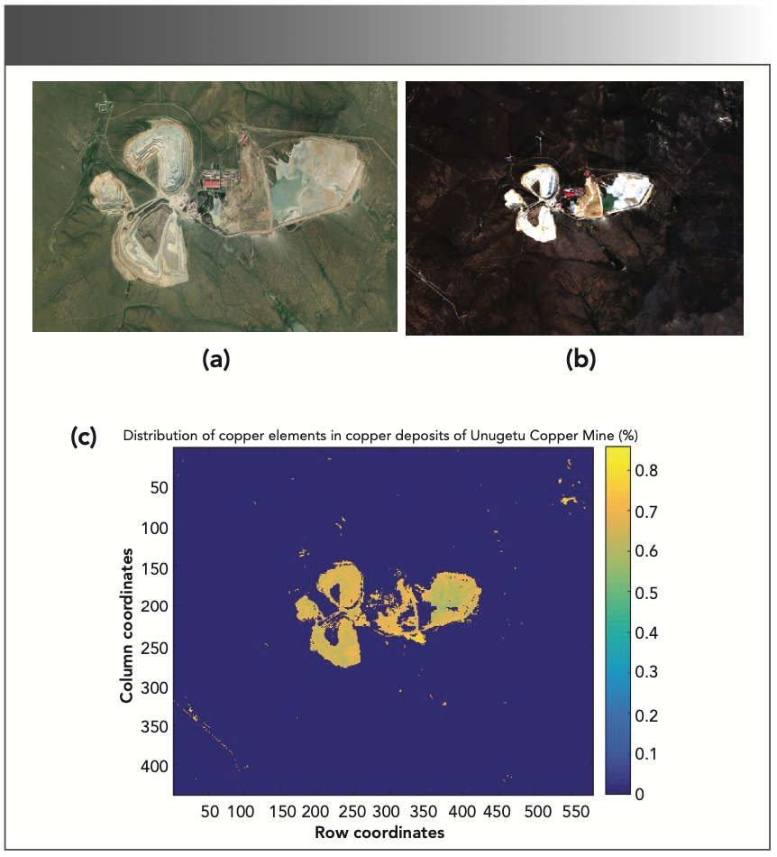
The Unugetu Copper Mine is located in the Hulunbuir Prairie in Manzhouli, Inner Mongolia. It is currently the first modern large-scale non-ferrous metal mine in the high and cold area of China. The Unugetu Copper Mine is open-pit mining. The latitude and longitude of the mining area is 117° 14’ -117° 22’ east longitude and 49° 22’ -49° 30’ north latitude. Figure 8a is a satellite image of the Unugetu Copper Mine.
Spectral Data
We collected 128 copper ore samples from the Unugetu Copper Mine, on August 20, 2017. We cleaned and dried the surface of the samples, and then grounded them into a powder. After the sample preparation was completed, we used the SVC HR-1024 portable spectrometer to perform spectrum experiments on each sample.
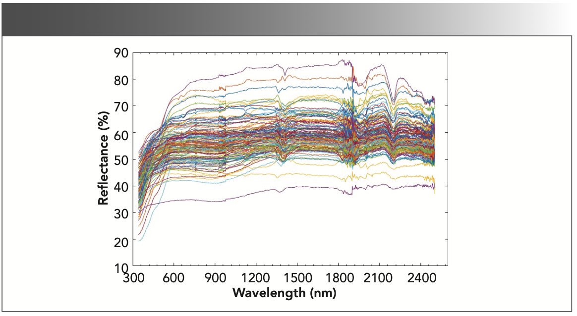
In the spectrum experiment, a white-board calibration was performed every ten replicates of the spectrum measurement. We conducted three replicate measurements on each sample to reduce measurement errors. We averaged the three replicates for each sample as its spectral data. After the completion of the spectrum measurements, the final spectral data of the copper ore for calibration was obtained by data preprocessing operations, such as coarsening and band fitting of the measured spectral data. Figure 1 shows the reflectance of copper ore samples at different wavelengths.
FIGURE 1: Spectral data for copper ore samples.
Remote Sensing Data
We downloaded Landsat-8 multispectral data from the U.S. Geological Survey website, and then used ENVI to perform radiometric calibration, atmospheric correction, image fusion, and other processing on the downloaded Landsat-8 multispectral data. Finally, as shown in Figure 8b, a multispectral image of the Unugetu copper mining area was obtained. Then used ENVI Class to extract the spectral data corresponding to each pixel in Figure 8b as the final remote sensing data.
Experimental Ideas
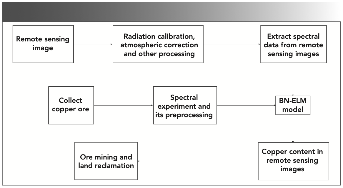
We used the spectral data in the training set as input and the copper content as output to train the BN-ELM model. The spectral data in the test set were then used as input to predict the content and evaluate the model. Finally, using the extracted remote sensing data as the input of BN-ELM model, the corresponding copper content of each pixel was obtained. The copper content of the whole min- ing area can be performed by this method, thus providing guidance for the mining and reclamation of the mining area in the future. The research idea is shown in Figure 2.
FIGURE 2: Flow chart of heavy metal inversion in the mining area.
Experimental Method
Extreme Learning Machine
ELM is a typical feedforward neural network that can initialize the input weights and biases randomly, and solve the output weights by the least square method. Suppose there are N arbitrarily different samples, where xi = [xi1, xi2, ..., xin]T ε Rn, ti [ti1, ti2, ..., tim]T ε Rm. The ELM calculation formula is:

In equation 1, ω is the randomly initialized input weight, bi is the random initialization bias, L is the number of hidden layer nodes set, g is the activation function, xj is the number of inputs for each sample, and βi is the weight of the output layer and the hidden layer. Simplify equation 1 to get:

And using equation 2, we expand it to equations 3 and 4,
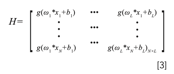
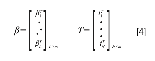
We solve equation 2 by the least squares method:

Using the two theorems proposed by Huang, we can get equation 6.

Where H+ is the inverse matrix of H obtained by SVD decomposition, and Huang proved that

exists and is unique.
Batch Normalization-Extreme Learning Machine
In the ELM algorithm, the activation function can introduce nonlinear factors into the model, possibly making the input and output a non-linear relationship. The activation function can also enable the neural network model to better solve complex problems and improve the generalization performance of the network. Commonly used activation functions are shown in Table I.
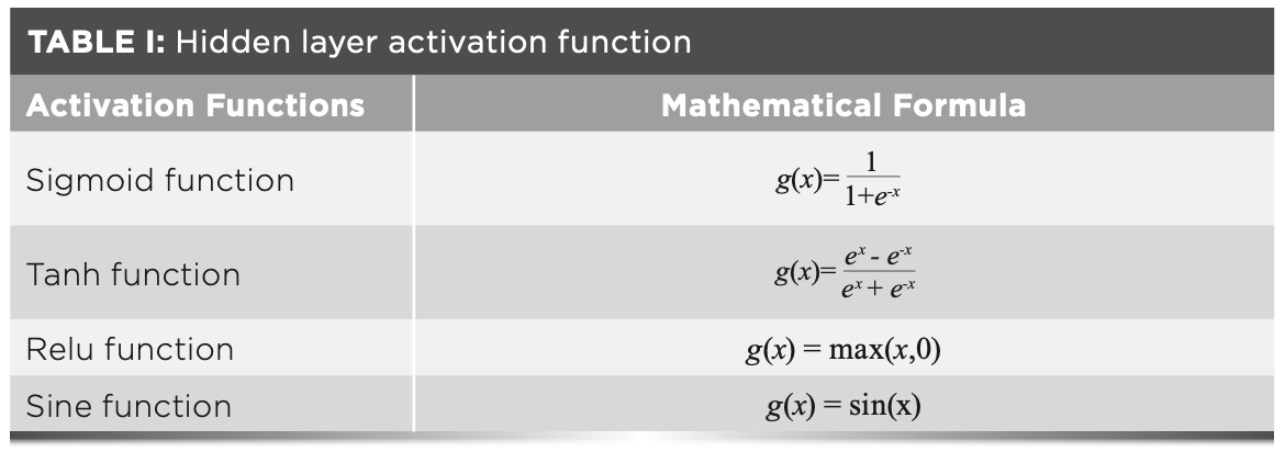
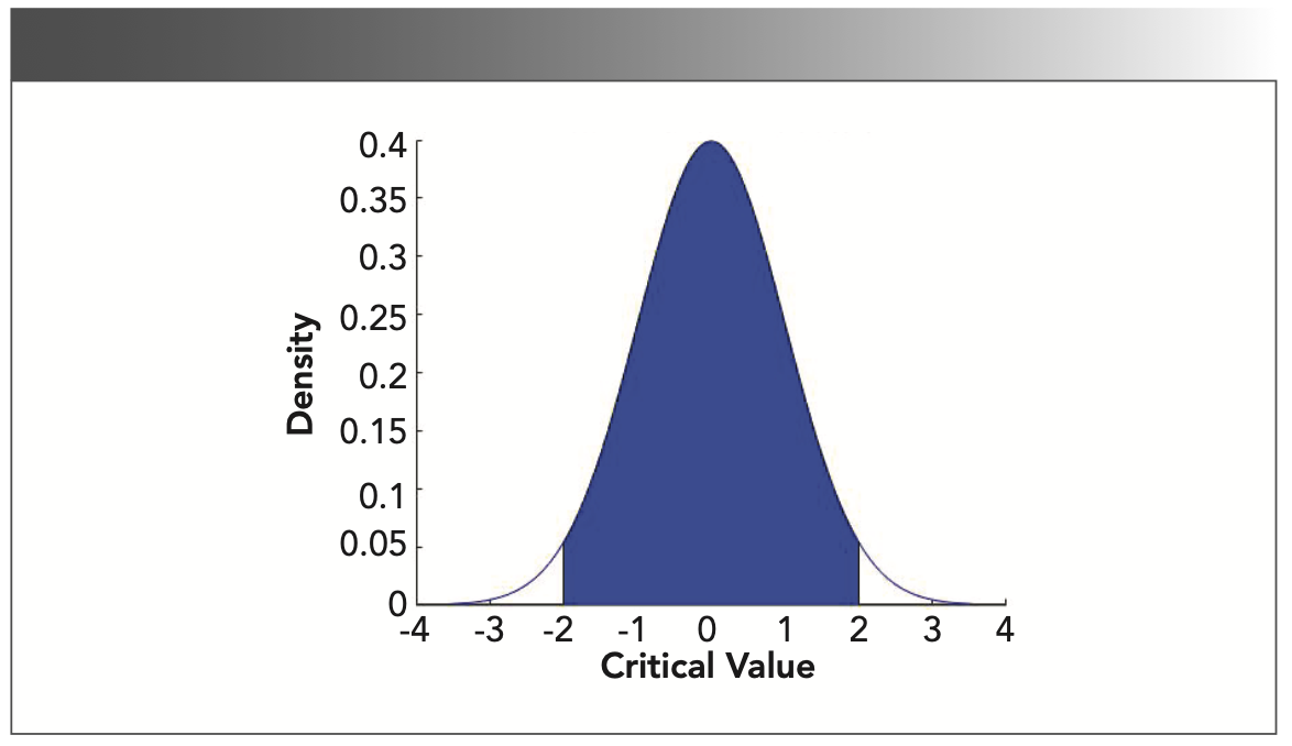
Sigmoid function (also known as logistic function) is used for the hidden layer neuron output, and its value range is (0,1). The graph of the sigmoid function presents an S-shaped curve. Because the output range of the sigmoid function is (0,1), the sigmoid function can be used to compress data, and is suitable for forward propagation. However, when the absolute value of the input variable is greater than 4, saturation will occur, and the output will become insensitive to small changes in the input. The tanh function is also called the hyperbolic tangent function, and its value range is [-1,1]. As shown in Figure 3; the tanh function also has saturation. By observing Figure 3, we found that when the absolute value of the input variable is greater than 4, the sigmoid and tanh function activation functions are close to output saturation. At this time, the output is not sensitive to subtle changes in the input. Using the rectified linear activation function (ReLU) will cause some neuron necrosis. At this time, the gradient of the neuron is 0, and no longer responds to any data. When the range of the input variable value is too large, the sine function is not a monotonic function.
FIGURE 3: Images showing activation functions from Table I.
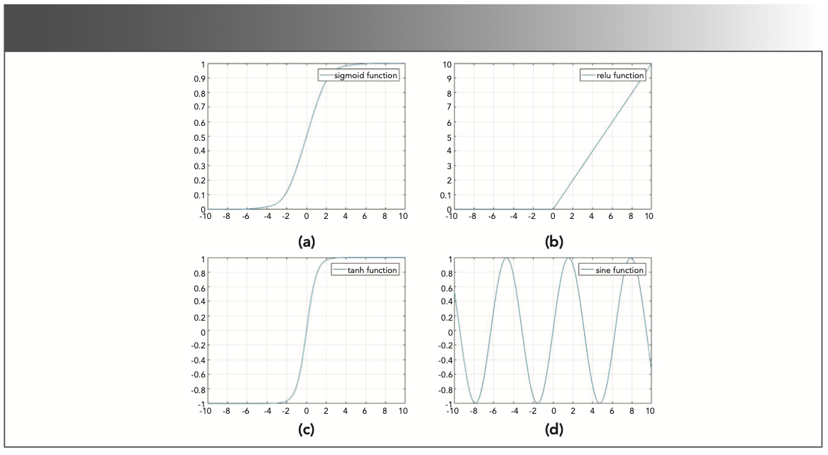
To solve the saturation problem, we added a BN layer in front of the hidden layer (32). Figure 4 shows the network structure of the BN–ELM. The BN layer can make the output of the hidden layer fall on a normal distribution with a mean of 0 and a variance of 1. It can be seen from Figure 5 that the probability that the value of each data is within [-2,2] is 95.45%. Therefore, the training of the BN layer can not only make the output of the hidden layer fall between [-2, 2] as much as possible, but can also avoid an internal covariate shift.
FIGURE 4: Illustration of BN-ELM network structure.
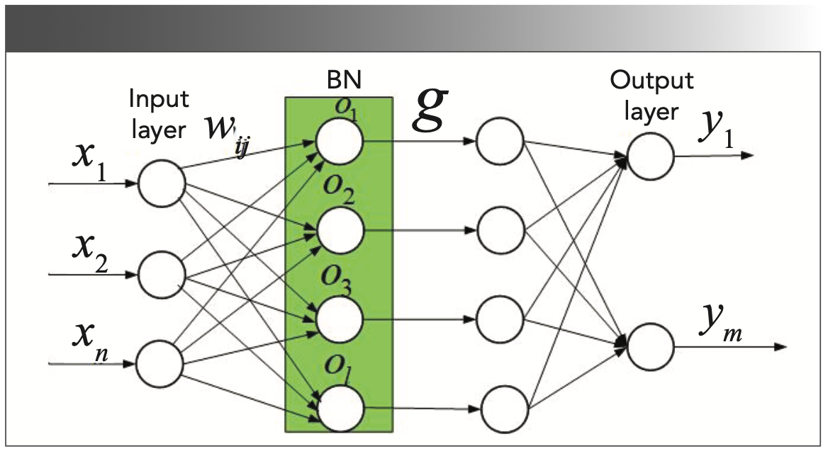
FIGURE 5: Illustration of standard Gaussian distribution probability density; probability between limits is 0.9545.
Algorithm Flow of BN–ELM
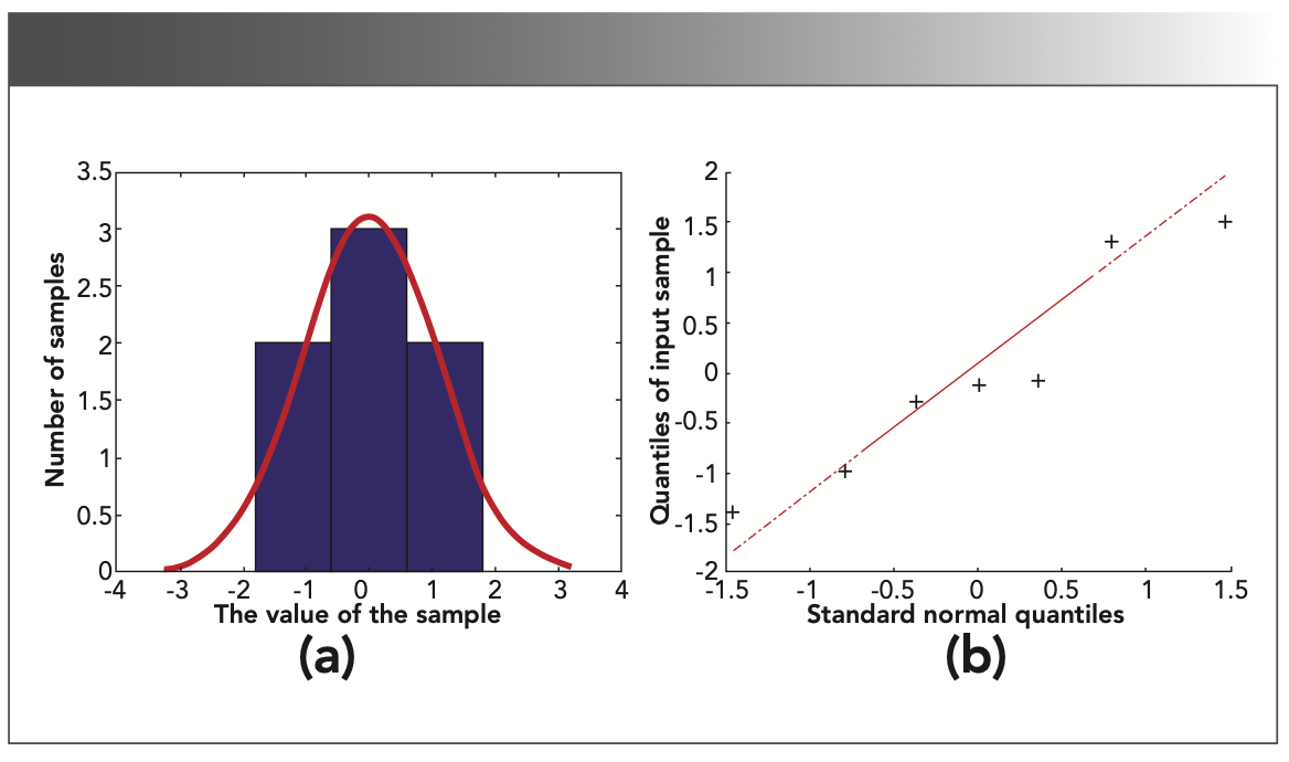
In the BN–ELM algorithm, first randomly generate weight w and threshold b that conform to a Gaussian distribution with a mean value of 0 and a variance of 1. Because the hyperspectral remote sensing data has only seven dimensions, we assume that the 7-dimensional data conforms to the Gaussian distribution, and then normalize the spectral data with a z-score. Figure 6a shows the distribution of spectral data after z-score normalization. Figure 6b is a Q-Q chart of spectral data. It can be seen from Figures 6a and 6b that the spectral data of each group obeys the standard Gaussian distribution.
FIGURE 6: (a) Sample distribution showing Gauss distribution test; (b) Q-Q diagram of the sample, showing a plot of sample data versus standard normal data.
Then, we assume that the spectral data conforms to a Gaussian distribution with a mean of 0 and a variance of 1, that is: X ~ N (μ1; σ12). We make the weight W and the threshold B also conform to the Gaussian distribution, namely: W ~ N (μ2; σ22), B ~ N (μ3; σ32). So TEH = WX + B also conforms to the Gaussian distribution, the proof is as follows.
According to the probability density function of Gaussian distribution, we can get:
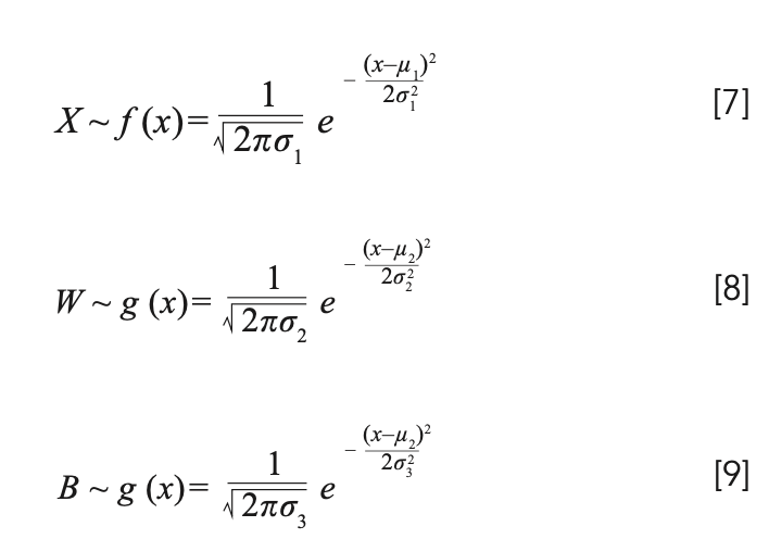
First, we prove that WX = g(x) f(x) conforms to Gaussian distribution. It can be inferred from equation 7 and equation 8:
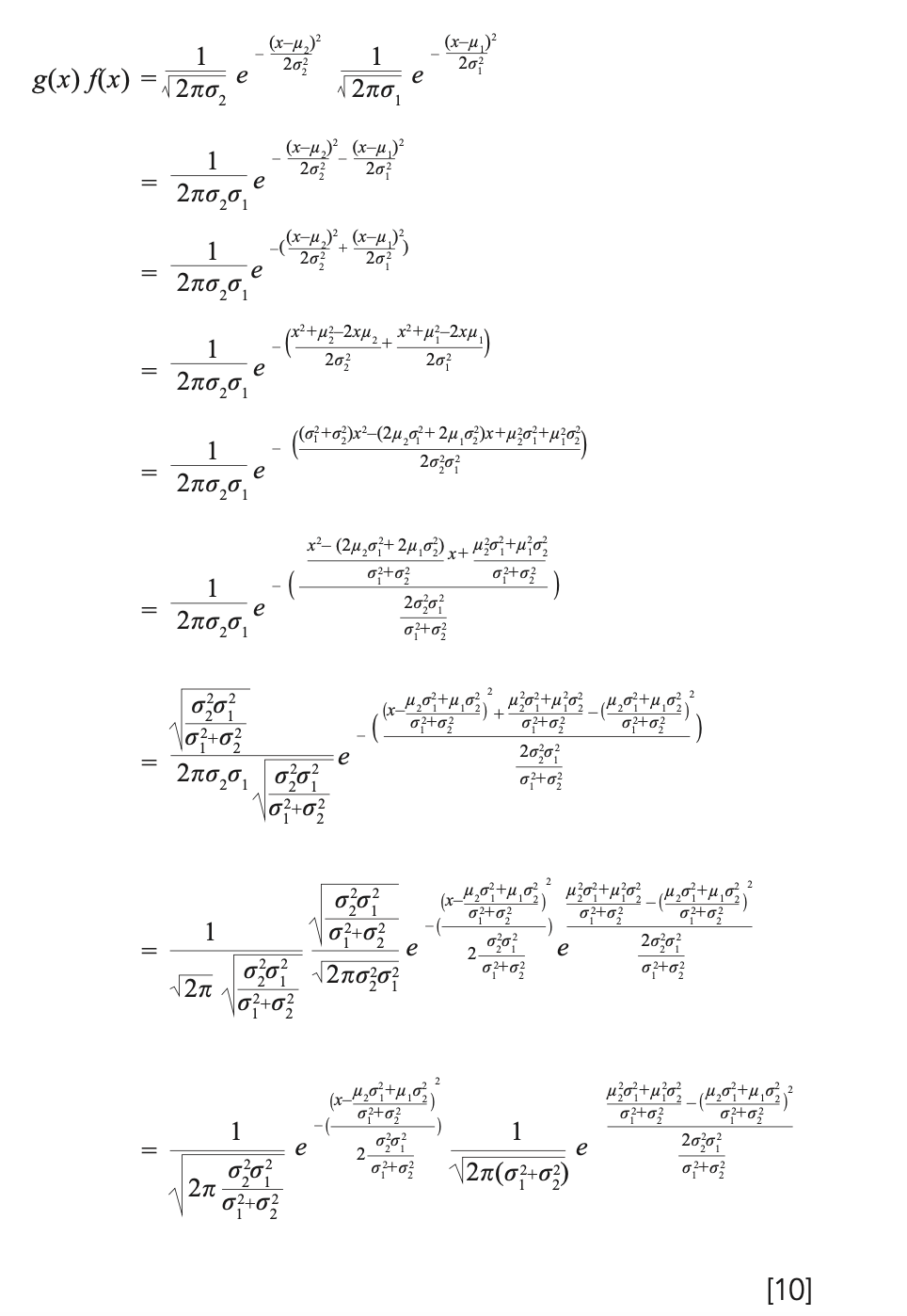
Let:


So, g(x) f(x) conforms to the Gaussian distribution with a scaling factor of ɑ:

Then:

From equation 14, we can find that, because of the calculation of the hidden layer fully connected, the output matrix TEH no longer conforms to the Gaussian distribution with the mean of 0 and variance of 1. We therefore performed batch normalization processing on TEH. First, we calculate the mean and variance of each hidden layer node.
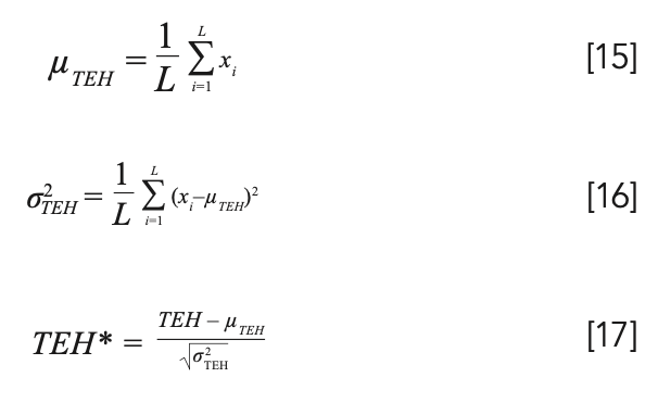
It can be inferred from equation 15 and equation 16 that, if the training sample is large enough, the mean and variance of the hidden layer nodes will be more stable. The mean and variance of the internal offset generated during the training of the training set can be used to replace the mean and variance generated by the internal migration of all data. Therefore, there is no need to recalculate the mean and variance of hidden layer nodes when testing on the test set. After batch normalization processing, the hidden layer matrix obeys a Gaussian distribution with the mean of 0 and the variance of 1.
The output matrix of the hidden layer with the same distribution as the original data is obtained. We then use the activation function to calculate the hidden layer matrix, and finally use the least square method to get the output weight β. After the calculation of the BN layer, not only can the hidden layer value fall within [-2,2] as much as possible, but it will also retain the characteristics of the original input.
Experimental Results and Discussion
Comparison of Neural Network Algorithms
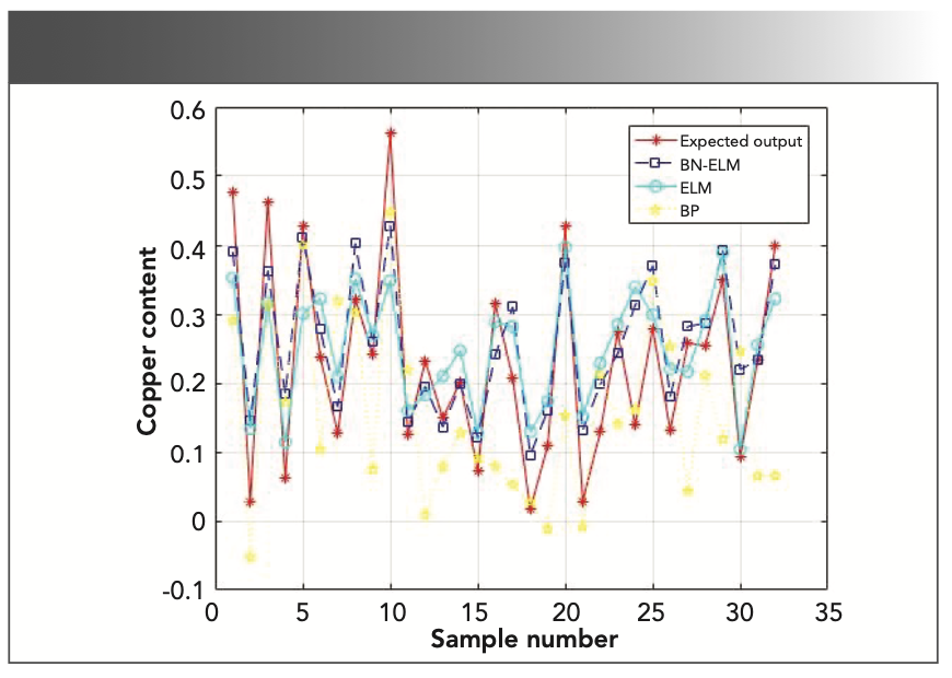
In this paper, four neural network algorithms of BP, RBF, ELM, and BN–ELM are used in the Matlab 2016a environment to compare and verify the feasibility of the BN–ELM algorithm. Multiple cross-validation methods were used for experiments to prove the stability of the BN–ELM algorithm. The experimental results are shown in Tables II and III. From these tables, it can be seen that the BP neural network can easily fall into the local optimal solution during the back propagation, so it presents an unstable phenomenon. The RBF neural network has the worst prediction result. The ELM does not need to calculate the weight w and the threshold b in reverse, so it will not fall into the local optimal solution. But in the ELM algorithm, because of the saturation of the activation function, the output is not sensitive to small changes in the input. BN–ELM solves the saturation problem of the ELM activation function, and keeps the hidden layer matrix within [-2,2] as much as possible. By comparison, it can be found that BN–ELM has the highest coefficient of determination and the smallest root mean square error. Figure 7 is a comparison of the best results of the cross-check.
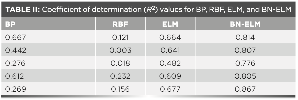
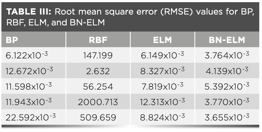
FIGURE 7: Comparison of copper ore content prediction results for various calculations versus actual (expected output in red).
Remote Sensing Inversion of Mining Area
We used NEVI Classic software to obtain all the spectral information in Figure 8b. Because we are using the Landsat 8 multi-spectral image, each pixel can extract the reflectance of seven bands, and each band corresponds to the spectrum of the copper ore collected from the Wunugetushan copper mine data. After BN–ELM simulation, the copper content corresponding to the whole Figure 8b is obtained. Finally, we plotted the copper content distribution of the entire mining area, as shown in Figure 8c.
FIGURE 8: (a) Satellite image of copper mining area; (b) remote sensing image of mining area; (c) remote sensing retrieval of copper content in Unugetu Copper Mine.
Conclusion
With the continuous mining of the area studied, high-grade ore has been exhausted. Therefore, attention should be paid to low-grade ores. However, the low-grade ore contains less ore and has low mining value, so it brings less benefit to enterprises. The traditional copper ore grade determination is costly and difficult to be determined in large quantities. This paper puts forward the method of using spectral information and BN–ELM modeling to analyze the grade of copper ore. This method has the advantages of high speed and low cost. Finally, we use Landsat 8 remote sensing data to analyze the content of the whole mining area, providing guidance for future mining and land reclamation.
References
(1) M. Radetzki, Resour. Policy 34(4), 176–184 (2009). DOI: 10.1016/j.resourpol.2009.03.003.
(2) M. Pearce, J. World Prehistory 32(3), 229–250 (2019). DOI: 10.1007/s10963-019- 09134-z.
(3) P. Fox, BioMetals 16(1), 9–40 (2003). DOI: 10.1023/A:1020799512190.
(4) X.Y. Ma, S. Jiang, S.M. Yan, M. Li, C.C. Wang, Y.G. Pan, C. Sun, L.N. Jin, Y. Yao, and B. Li, Biol. Trace Elem. Res. 197(1), 43–51 (2020). DOI: 10.1007/s12011-019-01979-x.
(5) S. Raha, R. Mallick, S. Basak, and A. K. Duttaroy, Med. Hypotheses 142, 109814 (2020). DOI: 10.1016/j.mehy.2020.109814.
(6) W.Q. Zhang, S.M. Fan, X.L. Li, S.Q. Liu, D.W. Duan, L.P. Leng, C.X. Cui, Y.P. Zhang, and L.B. Qu, Microchim. Acta 187(1), 69(2020). DOI: 10.1007/s00604-019-4044-y.
(7) K. Supong and P. Usapein, Water Sci. Technol. 79(5), 833–841 (2019). DOI: 10.2166/wst.2019.072.
(8) D. Yildiz and M. Demir, J. Anal. Chem. 74(5), 437–443 (2019). DOI: 10.1134/S1061934819050022.
(9) Z.Y. Li, Z.W. Ma, T.J. van der Kuijp, Z.W. Yuan, and L. Huang, Sci. Total Environ. 468, 843–853 (2014). DOI: 10.1016/j.scitotenv.2013.08.090.
(10) X. Guan and L.N. Sun, Appl. Mech. Mater. 675–677, 612–614 (2014). DOI: 10.4028/www.scientific.net/AMM.675-677.612
(11) S.A. Sadeq and A.P. Beckerman, Arch. Environ. Contam. Toxicol. 76(1), 1–16 (2019). DOI: 10.1007/s00244-018-0555-5.
(12) S. Khan, Q. Cao, Y.M. Zheng, Y.Z. Huang, and Y.G. Zhu, Environ. Pollut. 152(3), 686–692 (2008). DOI: 10.1016/j.envpol.2007.06.056.
(13) J.O. Duruibe, M.O.C. Ogwuegbu, and J.N. Egwurugwu, Int. J. Phys. Sci. 2(5), 112–118 (2007). DOI: 10.1142/S0218127407018087.
(14) P. Zhuang, M.B. McBride, H.P. Xia, N.Y. Li, and Z.A. Lia, Sci. Total Environ. 407(5), 1551–1561 (2009). DOI: 10.1016/j.scitotenv.2008.10.061
(15) M.H. Tan, X.B. Li, and C. Lu, Land Use Policy 22(3), 187–196 (2005). DOI: 10.1016/j.landusepol.2004.03.003.
(16) Y.P. Peng, Y.C. Chang, K.F. Chen, and C.H. Wang, Environ. Sci. Pollut. Res. 27(28), 34760–34769 (2019). DOI: 10.1007/s11356-019-07444-5.
(17) Z.M. Jin, S.Q. Deng, Y.C. Wen, Y.F. Jin, L. Pan, Y.F. Zhang, T. Black, K.C. Jones, H. Zhang, and D.Y. Zhang, Sci. Total Environ. 697, 134148 (2019). DOI: 10.1016/j.scitotenv.2019.134148.
(18) F.Y. Zhang and Y. Zhou, Soil Sediment Contam. 29(2), 246–255 (2020). DOI: 10.1080/15320383.2019.1702921.
(19) L.J.M. Morong and N.S. Aggangan, Philipp. J. Crop Sci. 44, 18–27 (2019).
(20) Q.H. Wu, K. Liu, C.Q. Song, J.D. Wang, L.H. Ke, R.H. Ma, W.S. Zhang, H.Pan, and X.Y. Deng, Sustainability 10(11), 3851 (2018). DOI: 10.3390/su10113851.
(21) W. Song, W. Song, H.H. Gu, and F.P. Li, Int. J. of Environ. Res. Public Health 17(6), 1846. DOI: 10.3390/ijerph17061846.
(22) K. Koruyan, A.H. Deliormanli, Z. Karaca, M. Momayez, H. Lu, and E. Yalcin, J. South. Afr. Inst. Min. Metall. 112(7), 667–672. DOI: 10.1134/S1062739148040235.
(23) E. Charou, M. Stefouli, D. Dimitrakopoulos, E. Vasiliou, and O.D. Mavrantza, Mine Water Environ. 29(1), 45–52 (2010). DOI: 10.1007/s10230-010-0098-0.
(24) Z. Wei, H. Hu, H.W. Zhou, and A. Lau, Pure Appl. Geophys. 176(8), 3593–3605 (2019). DOI: 10.1007/s00024-019-02152-0.
(25) Y.P. Liu, L.X. Zhu, and Y.Z. Zhou, Acta Petrol. Sin. 34(11), 3217–3224 (2018).
(26) B.T. Le, D. Xiao, Y.C. Mao, D.K. He, S.Y. Zhang, X.Y. Sun, and X.B. Liu, IEEE Access 6, 44328–44339 (2018). DOI: 10.1109/ACCESS.2018.2860278.
(27) G.B. Huang, Q.Y. Zhu, and C.K. Siew, IEEE Intl. Joint Conf. Neural Networks 2, 985–990 (2004). DOI:10.1109/ IJCNN.2004.1380068.
(28) G.B. Huang, L. Chen, and C.K. Siew, IEEE Transactions on Neural Networks 17(4), 879–892 (2006). DOI: 10.1109/TNN.2006.875977.
(29) G.B. Huang and L. Chen, Neurocomputing 70 (16–18), 3056–3062 (2007). DOI: 10.1016/j.neucom.2007.02.009.
(30) H.J. Rong, Y.S. Ong, A.H. Tan, and Z.X. Zhu, Neurocomputing 72(1–3), 359–366 (2008). DOI: 10.1016/j.neucom.2008.01.005.
(31) Y. Miche, A. Sorjamaa, P. Bas, O. Simula, C. Jutten, and A. Lendasse, IEEE Transactions on Neural Networks 21(1), 158–162 (2010). DOI:10.1109/TNN.2009.2036259.
(32) S. Ioffe and C. Szegedy, Intl. Conf. on Machine Learning, PMLR 37, 448–456 (2015). arXiv:1502.03167.
Dong Xiao and Hongfei Xie are with the Information Science and Engineering School at Northeastern University, in Shenyang, China. Yanhua Fu is with JangHo Architecture College at Northeastern University, in Shenyang, China. Feifei Li is with the Liaoning Province Important Technology Innovation and R & D Base Construction Engineering Center in Lialong Province, China. Direct correspondence to: Dong Xiao at xiaodong@ise.neu.edu.cn ●

NIR Spectroscopy Explored as Sustainable Approach to Detecting Bovine Mastitis
April 23rd 2025A new study published in Applied Food Research demonstrates that near-infrared spectroscopy (NIRS) can effectively detect subclinical bovine mastitis in milk, offering a fast, non-invasive method to guide targeted antibiotic treatment and support sustainable dairy practices.
New AI Strategy for Mycotoxin Detection in Cereal Grains
April 21st 2025Researchers from Jiangsu University and Zhejiang University of Water Resources and Electric Power have developed a transfer learning approach that significantly enhances the accuracy and adaptability of NIR spectroscopy models for detecting mycotoxins in cereals.
Karl Norris: A Pioneer in Optical Measurements and Near-Infrared Spectroscopy, Part II
April 21st 2025In this two-part "Icons of Spectroscopy" column, executive editor Jerome Workman Jr. details how Karl H. Norris has impacted the analysis of food, agricultural products, and pharmaceuticals over six decades. His pioneering work in optical analysis methods including his development and refinement of near-infrared spectroscopy, has transformed analysis technology. In this Part II article of a two-part series, we summarize Norris’ foundational publications in NIR, his patents, achievements, and legacy.
New Study Reveals Insights into Phenol’s Behavior in Ice
April 16th 2025A new study published in Spectrochimica Acta Part A by Dominik Heger and colleagues at Masaryk University reveals that phenol's photophysical properties change significantly when frozen, potentially enabling its breakdown by sunlight in icy environments.