Soil Organic Matter Estimation Modeling Using Fractal Feature of Soil for vis-NIR Hyperspectral Imaging

To produce a fast, accurate estimation for soil organic matter (SOM) by soil hyperspectral methods, we developed a novel intelligent inversion model based on multiscale fractal features combined with principal component analysis (PCA) of hyperspectral data. First, we calculated the local generalized Hurst exponent of the spectral reflectivity by multiscale multifractal detrended fluctuation analysis (MMA) while determining the sensitive spectral bands. PCA was employed to access the maximum principal component features of the sensitive bands used as the model input. Finally, two intelligent algorithms, random forest (RF), and a support vector machine (SVM), were utilized for establishing the SOM estimation model. The soil hyperspectral data possesses the typical nature of long-range correlation, presenting distinct fractal structures at different scales and fluctuations. The sensitive bands were from 359 nm to 405 nm, and were not impacted by window fitting size. The accuracy of the models of MMA-based sensitive bands is superior to that of the original bands. The PCA processing brings additional model performance improvement. The MMA-based models combined with RF is recommended for SOM estimation.

As the critical indicators to assess soil fertility, soil organic matter (SOM) provides essential nutrient and energy for plant and microbial life activities (1). Determining SOM content is an important task that is normally measured in laboratory. Although the laboratory method produces high precision, it is not conducive to real-time measurement. Developed in the 1980s, hyperspectral technology brought about a revolution in the field of remote sensing (2,3), which is widely applied in soil science. Owing to the effect of the absorption of SOM and its reflect spectral properties, the soil hyperspectral data expresses the comprehensive presence of various physical and chemical properties. Accordingly, the hyperspectral data determination-based method has dominated SOM estimation modeling. Because of the potential information redundancy between the spectral bands, the spectral reflectivity may overlap with other physical and chemical properties (4). Therefore, knowing how to extract the effective features of the soil hyperspectral data reflectivity is a key point before SOM modeling.

Considering the fact that the spectral reflectivity involves the information on SOM as well as the moisture and impurities data, a strong redundance exists among the bands, which makes the reflectivity curve nonlinear and nonstationary. Therefore, extracting the spectral features accurately is of utmost importance. A number of novel methods were proposed for soil hyperspectral feature extraction. Zhu and associates (5) introduced a method of uninformative variables elimination and competitive adaptive reweighted sampling to locate the sensitive bands for the SOM. To make hyperspectral low-dimensional data preserve the spectral information more completely, Wu and colleagues (6) developed a band selection method based on the optimal linear prediction of principal components in subspace. For the purpose of estimating SOM based on correlation analysis, Bao and associates (7) used wavelet decomposition and the random forest (RF) method to determine the maximum wavelet decomposition layer and filter the sensitive bands. However, determining the sensitive band of these methods depends on the SOM content, which may lead to unstable results because of the laboratory determination error of the SOM.

Noting that the soil hyperspectral data contains different information in different bands, there may be changes (mutations and redundancy) between two adjacent bands. Multifractal theory (8) provides a different perspective to uncover the singularity of objects. With its advantage of being good at capturing the subtle changes of spectral data curves, multifractal theory is naturally applied to the field of spectral feature extraction (9–15). One of the feature extraction tools used most is detrended fluctuation analysis (DFA) (16,17), which was proposed to deal with various nonlinear measures in real world data (18,23). The estimated generalized Hurst exponent has become an important indicator to measure the log-term correlation of the object. However, the single-scale index is not enough to describe the change of correlation on different scales. To make up for this drawback, Gieraltowski and colleagues (24) proposed a multi-scale multifractal detrended fluctuation analysis (MMA) and obtained a set of scale-dependent Hurst exponents by introducing a moving fitting window traversing the entire spectral scale range. Using this method allowed the set of Hurst exponents to describe the richer dynamic behavior of the objects. Then, this method was applied to various applications (10, 25–30). By using the MMA as described in the literature (10), the authors developed a method to find the sensitive bands of the rapeseed spectrum according to the mutation point. They then utilized the multifractal feature of sensitive bands to establish a chlorophyll content estimation model. The result shows that the new method performed better than traditional methods. Compared to other methods of spectral analysis, the MMA focuses on the change of correlation of the spectral reflectance between the bands, and it allows capture of the mutation of the reflectivity information, which can help to determine the sensitive band.

As mentioned previously, sensitive bands selection is an effective hyperspectral dimensionality reduction method (6), which is a key preliminary work of modeling. The idea of MMA provides a new approach for finding sensitive bands (10). However, there may still be redundant information in sensitive bands. In this case, principal component analysis (PCA) can help to eliminate redundancy efficiently when used only on the relative short-band spectral range. With the idea of combining MMA and PCA, we first identify the sensitive bands for the soil hyperspectral reflectivity by using the MMA, and then conduct the PCA on the sensitive bands to obtain the first few principal components. Finally, using the principal components as the model input, we build regression models based on intelligent algorithms to be determined for SOM estimation.

The rest of this paper is organized as follows:

• Section 2 gives data acquisition.
• Section 3 offers a brief review of the MMA method and two intelligent regression modes: random forest and support vector machine.
• Section 4 provides a first study of the multifractal nature of the soil hyperspectral samples and conducts MMA on them (subsection 4.1), and then determines the sensitive bands for them (subsection 4.2). Next, PCA is conducted on the sensitive bands to obtain a few principal components (subsection 4.3). Finally, subsection 4.4 shows the performance of the SOM estimation models.
• Section 5 summarizes the full text.

Materials

Regional Situation

The paddy soil samples collected from Changsha and its surrounding areas in Hunan Province (112.608–114.067 °E, 27.536–28.514 °N) with flat terrain. The soil is well-drained, and the pH is between 4.5 and 9.0. The soil profile (depth 0–130 cm) of each sampling point contains 5–7 layers.

Sample Collection and Spectral Determination

By using a handheld GPS positioning instrument, we collected 79 paddy soil samples randomly from 13 profiles of the studied area. After air-drying and grinding the soil samples in the laboratory, each sample was divided into two parts, one for spectral determination and another for physical and chemical properties analysis.

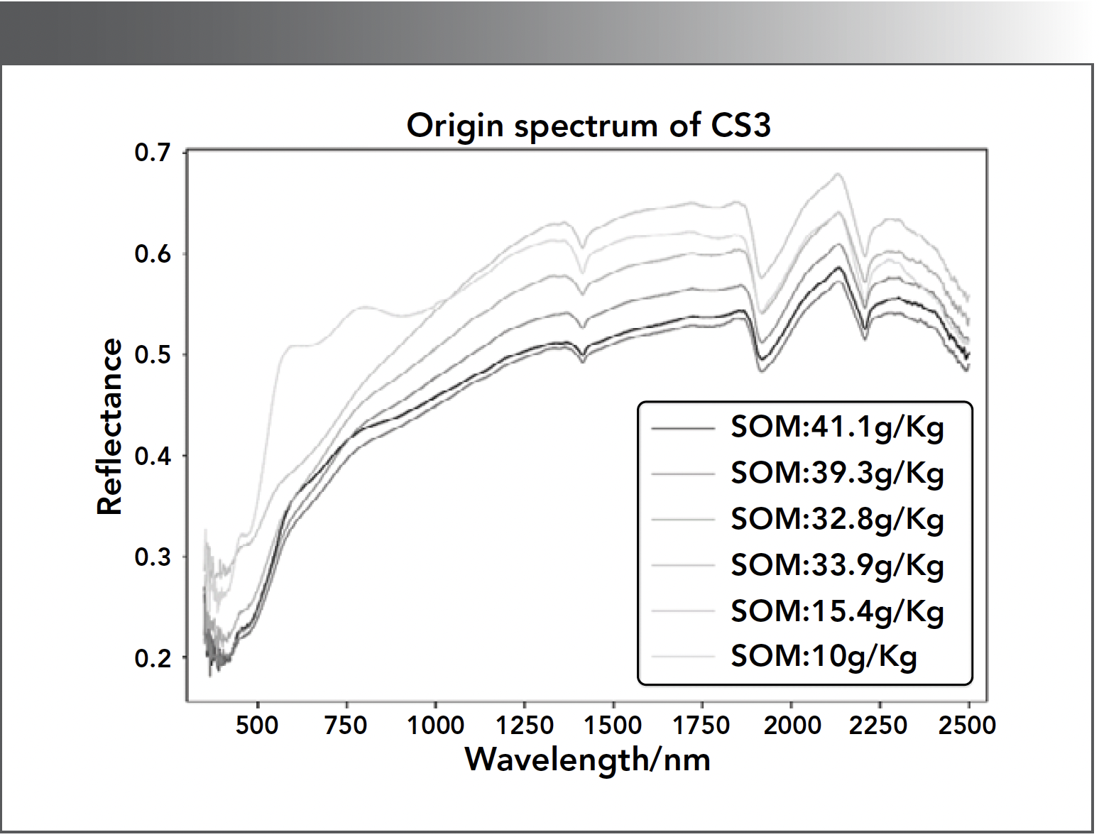
The spectra of the soil samples were collected by using a visible near-infrared (vis-NIR) spectrometer (ASD Vis-NIR). The wavelength range was 350–2500 nm. The sampling interval was 1.4 nm in 350–1000 nm and 2.0 nm in 1000–2500 nm, with a resampling interval 1 nm. The number of every spectral band is 2151. Taking sample CS03 as an example, there are six layers, the corresponding SOM content (unit: g/kg) being 41.1, 39.3, 32.8, 33.9, 15.4, and 10. Figure 1 shows their hyperspectral reflectivity. It is observed that the shape of the reflectivity curves is similar for different layers and the reflectivity is inversely proportional to the SOM content.

FIGURE 1: Spectral reflectance of soil samples with varying Soil Organic Matter (SOM) content. Six soil samples with distinct SOM content are analyzed at sampling point CS03, each represented by curves of different colors.

The SOM content was measured by a potassium dichromate-external heating method; each were obtained by averaging over twice determination. The following SOM estimation model was trained on a training set (choose a certain number of samples at random), whereas the model performance was evaluated on a testing set (the remaining samples).

Methods

MMA

The well-known multifractal DFA (MF-DFA) (17) method is an effective solution of nonstationary measure. The estimated generalized Hurst exponent can describe the global long-term correlation. However, in the real world, the series always exhibits various correlations at different scales. The change of the correlation may cause mutation point or crossover (31), which interferes with the judgement of the global correlation. Unfortunately, MF-DFA cannot detect this phenomenon. To solve this problem, multiscale MF-DFA (abbreviated as MMA) (24) was designed as a “crossover finder,” which estimates local Hurst exponents in a moving fitting window over the whole series. In this way, the crossover will be easy to find out, and different correlations can be detected at different scales. The first three steps of MMA are the same as the MF-DFA, shown as follows:

Step 1: For a real-world series (in our work, it is the soil hyperspectral reflectivity sequence), {x_i} (i = 1, 2, …, N, N is the spectrum wavelength), the profile is calculated by

Divide the {X_k} into N_s = [N/_s] non-overlapping subsequences with the size length s. Because the N is not always an integer multiple of s, the {X_k} is reversed and implemented the same division so as not to omit a few points at the series tail. Hence, 2N_s subsequences are obtained. For each subsequence v (v = 1, 2, …, 2N_s), the residual sequence Y_s(k) is generated by detrending the local trend (usually using polynomial fitting; in this work, we take 1-order fitting) from the profile.

Step 2: Calculate the variance in each interval v

Then, the average q-order fluctuation function over all the considered intervals can be determined by:

F (q, s) can be considered the weighted fluctuations for all the intervals. The F (q, s) with q < 0 describes the fluctuation of those intervals in which the signal has a low variance (the small fluctuation intervals mainly refer to the noise bands for the hyperspectral signal), whereas for q > 0, it characterizes the fluctuation of the larger variance intervals (17).

Step 3: For each given q, varying the scale s, the global long-term correlation of the original {x_i} can be determined by the power-law between the F (q, s) and s:

for q ≠ 0 (F_q(s) = exp {F (q, s)} ~ s^h(q) for q = 0). The h(q) is so-called generalized Hurst exponent, which can be estimated by the gradient of those two quantities in the double log-plot. Generally, the h(q) depends on q if the series possesses multifractal nature.

Above is the process of traditional MF-DFA. There is an extra step for the idea of MMA, which is described below.

Step 4: To obtain the local correlation at different scale, a moving fitting window is introduced to slide over the F_q(s) (14,29). In each window, the q-dependent local-scale exponent h(q, s_Ri) is calculated by:

where F_q(s)_Ri and s_Ri represent the q-order fluctuation function and scale in the window R_i, respectively. There are two critical factors of the fitting window, namely, the window length (WL) and the sliding length (SL). To traverse all the values of F_q(s), the value range of the starting point of the window takes the interval [s_min, s_max] with the SL, and the window length equals the starting point multiplying the WL. The fitting accuracy of h(q,s_Ri) is highly dependent on the WL, and the SL determines the number of the local-scale exponents. When the fitting window traverses the whole scale range, a series of h(q,s) is obtained. The h(q,s) appears in space as a curved surface that depends on q and s, whose shape reflects the long-term correlation of the studied series at different scales and fluctuation intervals.

Modeling Method

Random forest (RF) is a currency intelligent algorithm using multiple decision trees to train samples. With an idea of packing several decision trees together, RF averages the values of the outputs over every decision tree, which is predicted separately. Compared with the single decision tree, the RF algorithm randomly selects a feature on each node other than from the best node generated by each decision tree (32). Hence, RF has a good ability to explain nonlinear problems. With this advantage, RF is widely applied to both regression and classification (33).

Support vector machine (SVM) is also an intelligent algorithm to achieve classification or prediction through separating the samples with the best hyperplane. The idea of SVM is to map the samples to a higher-dimensional feature space in the case of not linearly separable in the lower-dimensional space. The key point of the SVM is to choose suitable kernel function (32). In this work, radial basis kernel function is chosen to our consideration.

Results

MMA of Soil Spectral Reflectivity

In the process of calculating the Hurst exponent by MMA (subsection 3.1), the value of q should be cautiously chosen. In references (24) and (29), the authors pointed out that the results for negative q should be used with caution since that q < 0 may produce much more unstable results with larger errors relative to positive q. Generally, we should not choose too large a q for a short length of series because of the divergence. Because there are 2151 bands of the sampling hyperspectral, the q is set 0.5, 1, 1.5, and 2 in this work. Besides the choice of q value, the range of scale s should also be considered in detail. In reference (17), the authors suggest that maximum of s should be less than N/4 (where N is the series length), which can be obtained the best scale-free interval for estimating the Hurst exponent. After checking the multifractality at different scales, we find that it is appropriate to set the range of scale s as [10, N/4]. Given N = 2151 and the WL = 4 and SL = 4, the fitting window from the start to the end is [10, 40], [14, 56], …, [130, 520]. After calibrating the scale of the coordinate axis s with the midpoint of the fitting window, its value ranges from 25 (the midpoint of the first window [10, 40]) to 325 (the midpoint of the [130, 520]). Seen from Figure 2a (taking sample CS-03-Aa as an example), the nice straight lines of the F_q(s) versus s in the double-log plot illustrates that the sample spectra of CS03 possesses typical fractal structure. The different gradient between the lines implies the multifractal nature.

FIGURE 2: Fractality of the spectrum of sample CS-03-Aa. (a) Double-log plot of F_q(s) versus s. (b) Local Hurst exponent h (q, s).

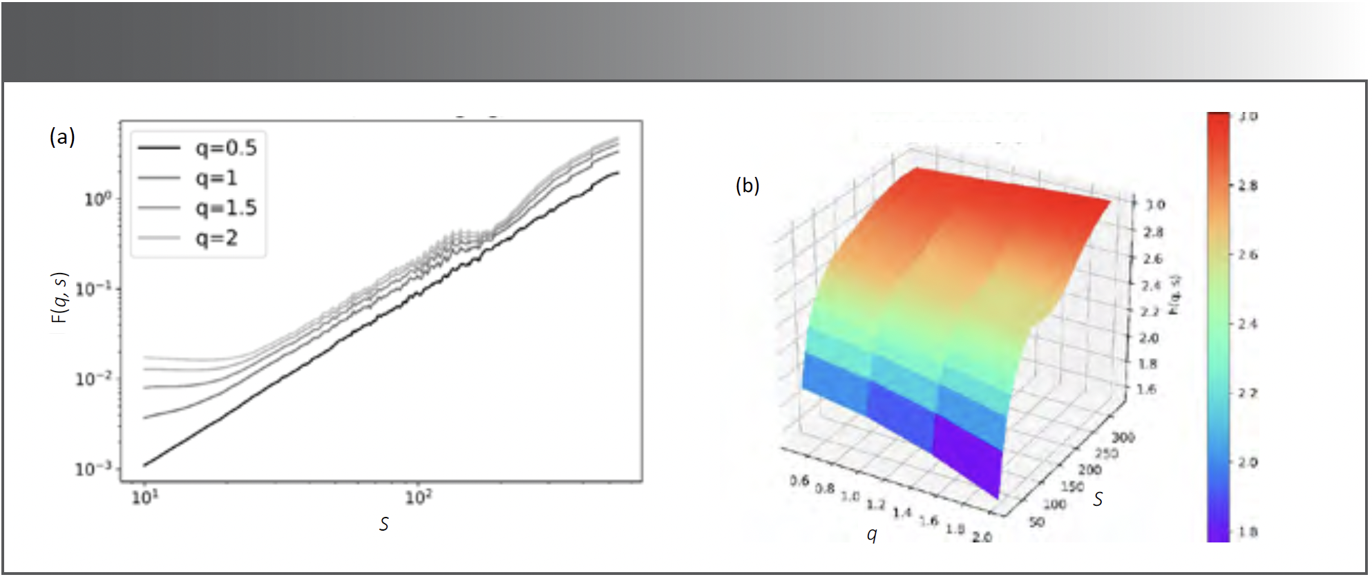
However, carefully observing Figure 2a, there is some difference of the gradient at different scales, which explains why crossovers may exist in those lines. In this regard, the global Hurst exponent h(q) cannot be the spectral characteristic for subsequent modeling. To show it more clearly, we draw the h(q,s) surface for the given q and s, as shown in Figure 2b. The steep obliquity (the lowest of h(q,s) locates at 1.8 and the highest locates at 3.0) suggests that there is significant difference between the local Hurst exponents at different bands. In this token, the true autocorrelation of soil spectrum should be represented by the h(q,s). Compared with the h(q,s) for the given q and s, the variation range of h(q,s) is the widest in the case of q = 2, which reflects the difference between the various spectral bands most significantly.

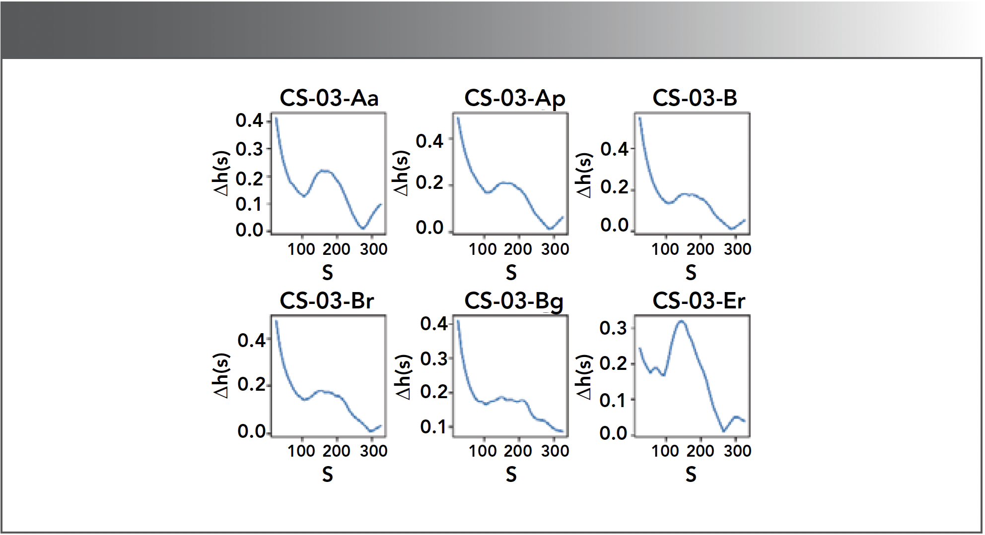
In addition, the multifractality at different scales also presents non-negligible difference, which can be depicted by defining ∆h(s) ≡ max_q (h(q,s)) – min_q (h[q,s]), as shown in Figure 3. Six subplots denote six levels of the soil sample CS-03. The change of ∆h(s) with respect to s exhibits the fractal structure is quite different for the various levels of the sample. The larger the ∆h(s) is, the more strength of the multifractality will be expected. The maximum ∆h(s), except for the level of CS-03-Er, are located at s = 25 and 35 (the corresponding original spectral bands are 359–405 nm). In general, the crossovers are more likely to occur at s where the multifractal strength is larger. Accordingly, we extrapolate that the sensitive bands of the soil spectrum may be the crossovers of the fractal structure.

FIGURE 3: Multifractal characteristics variation across different fitting windows. Δh(s) = max_q(h(q,s)) - min_q(h(q,s)) is with respect to the length of fitting window s. The six samples originate from sampling site CS03 at various soil depths.

Sensitive Bands Selection

On the basis of the local Hurst index of the soil spectrum obtained in the previous section, the sensitive bands can be found by the largest correlation between h(q,s) and SOM content. Specifically, for each q, the correlation coefficients between the h(q,s) and SOM content are calculated in different fitting windows, as shown in Figure 4. The sensitive band corresponds to the maximum correlation coefficient. Shown in Figure 4, the scales with the maximum correlation coefficient are 35, 25, 25, and 35, respectively for q = 0.5, 1, 1.5, 2, which is consistent with the extrapolation from Figure 3. The corresponding fitting windows are [14, 56], [10, 40], [10, 40], and [14, 56], and the bands of the original spectrum are 363–405 nm, 359–389 nm, 359–389 nm, and 363–405 nm, respectively. With comprehensive consideration, the sensitive bands of the soil spectrum are identified to be 359–405 nm.

FIGURE 4: Absolute value of the correlation coefficient (|corrcoef|) between h(q,s) and SOM content. Here, q denotes the order of the average fluctuation function. With q values of 0.5, 1.0, 1.5, and 2.0, the four subplots depict the trend of |corrcoef| as the length of the fitting window s varies.

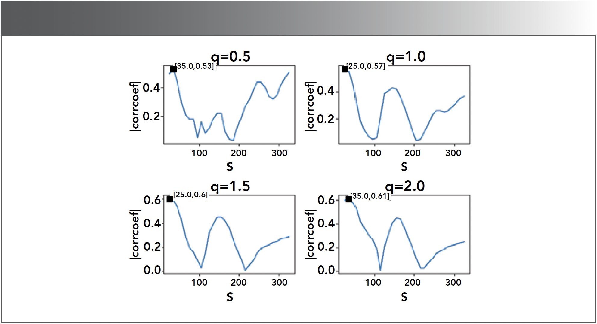
To test the stability of the extracted sensitive bands by MMA, different combinations of {WL, SL} are set. Table I lists the result. It shows that the sensitive bands are rarely affected by the parameter combination, which is basically stable at 359–405 nm, and the maximum correlation coefficient is approximately 0.6 obtained in the case of q = 2. In view of the robustness of the determined sensitive bands, we establish the SOM estimation based on the bands 359–405 nm.

PCA of Spectral Reflectivity in Sensitive Bands

Hyperspectral has the advantage of high resolution, ultra-long band ranges reflecting more thorough information for the object in the real world; however, the redundancy is inevitably existing in adjacent bands. PCA is an effective method to reduce the dimension of data, expressing the original data information with a few uncorrelated principal components by sacrificing trivial information. To eliminate the redundancy of spectral reflectivity, PCA is employed to perform on both the sensitive bands and the original spectrum bands. The contribution rates of the first three principal components (PC) are listed in Table II.

Noting that the contribution rate of the first principal component is more than 99.9% for the sensitive bands, which is 12.98% higher than that of the original spectrum, it is explained that the information content of the first principal component of the sensitive bands is richer than that of the original bands. Considering that nearly all the information content of the sensitive bands is concentrated in the first principal component, we used the first principal component of the sensitive bands as the characteristic for follow modeling.

Model Evaluation

To test the effectiveness of the sensitive bands as well as the necessity of the PCA processing, four comparison models were established to our consideration. Namely, the model input was the spectral reflectivity of original bands or sensitive bands, with PCA processing or without PCA, denoted as Origin-◊, Origin-PCA-◊, MMA-◊, and MMA-PCA-◊, respectively, with ◊ representing the two intelligent regression algorithms of RF and SVM. The model output was the same (the normalized SOM content). According to the contribution rate in the PCA for the model Origin-PCA and MMA-PCA, we used the first three principal components and the first principal component, respectively, as the model input. The above models were conducted on both the training and testing set. Two evaluation indicators of determination coefficients (R²) and root mean squared error (RMSE) were used to evaluate the model performance. The larger R² and smaller RMSE expressed better model performance.

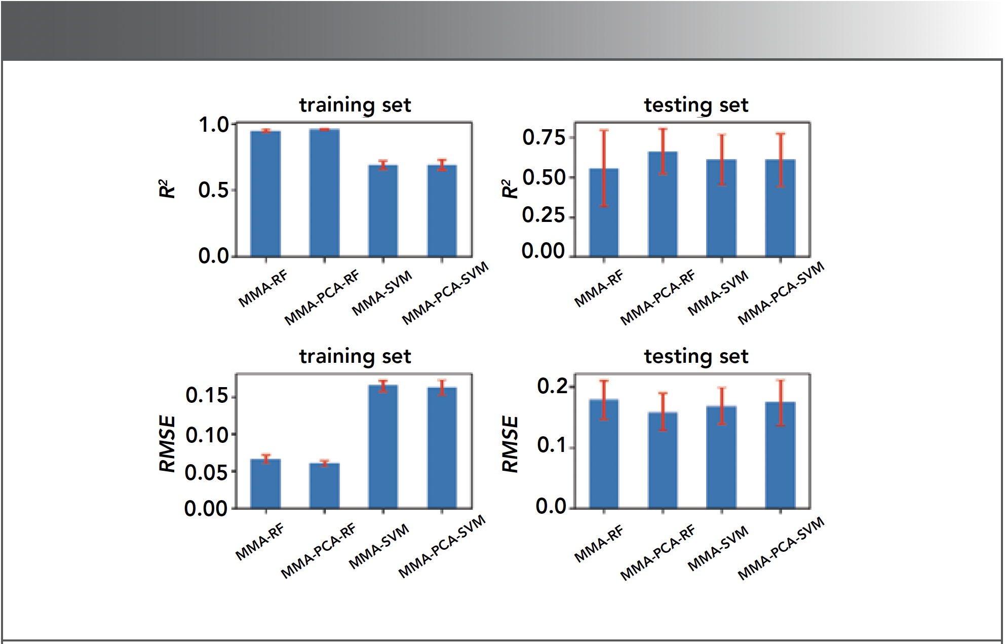
To verify the stability of the proposed models, four different numbers of training set were considered. Namely, 47, 55, 63, and 71 samples (the corresponding ratio is 60%, 70%, 80%, and 90%, respectively) were randomly selected to train these models. The results were averaged over 100 repetitions. The averaged R² and RMSE are shown in Figure 5. It is clear that the influence of the number of training samples on model performance is negligible. Figure 6 illustrated the results (the mean value together with the standard deviation) on the training set and testing set in the case of 63 training samples (80%). The effect on the whole is satisfactory, though the fluctuation of the results on the testing set was stronger than that on the training set. Comparing it to the models by using SVM, the performance of the RF-based models is slightly better; MMA-PCA-RF possesses the highest R² and the lowest RMSE along with the smallest fluctuation on the testing set.

FIGURE 5: The average results with different number of samples in training set.

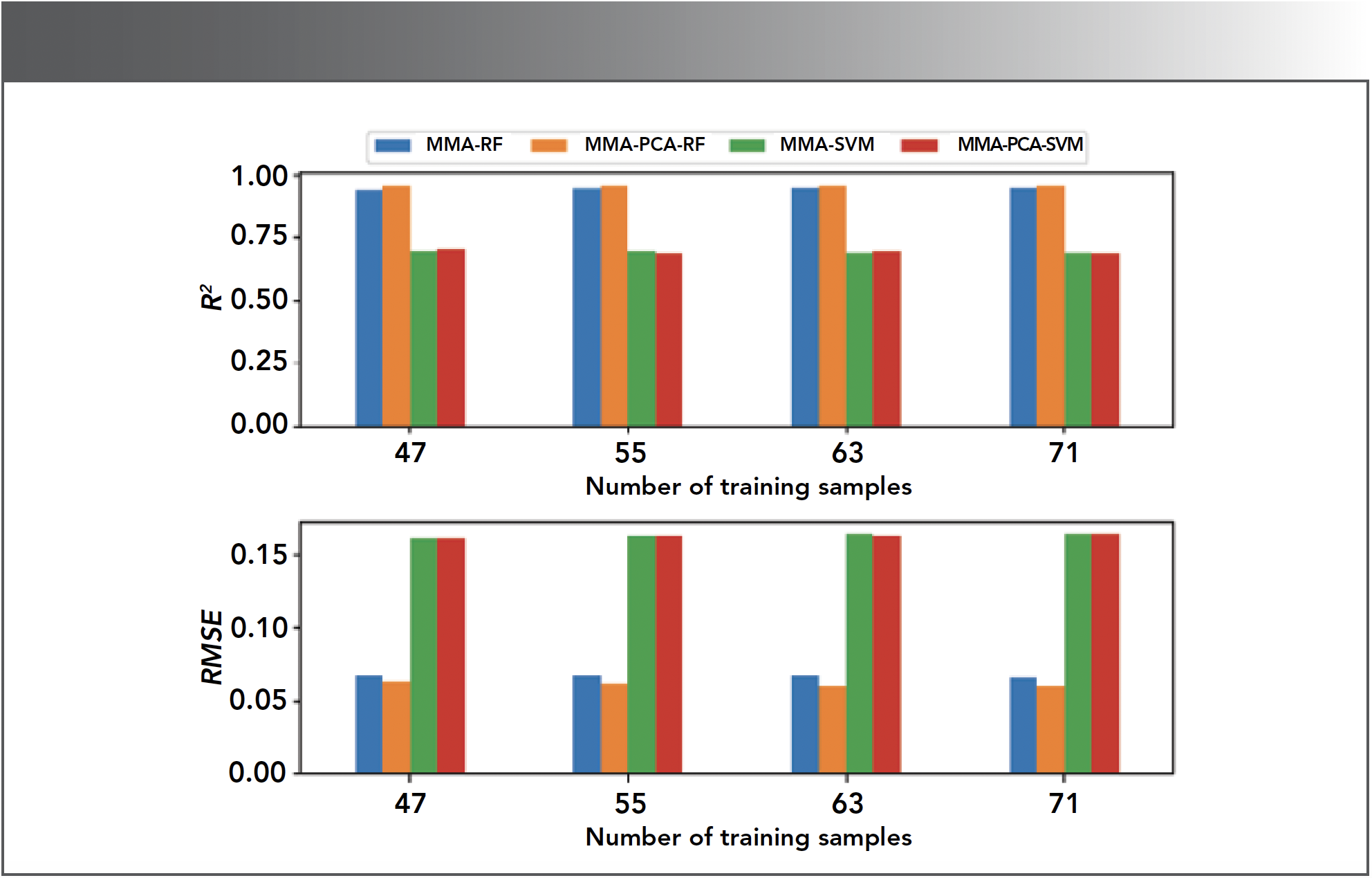
FIGURE 6: The average result and the standard deviation on training set (80%) and testing set (20%).

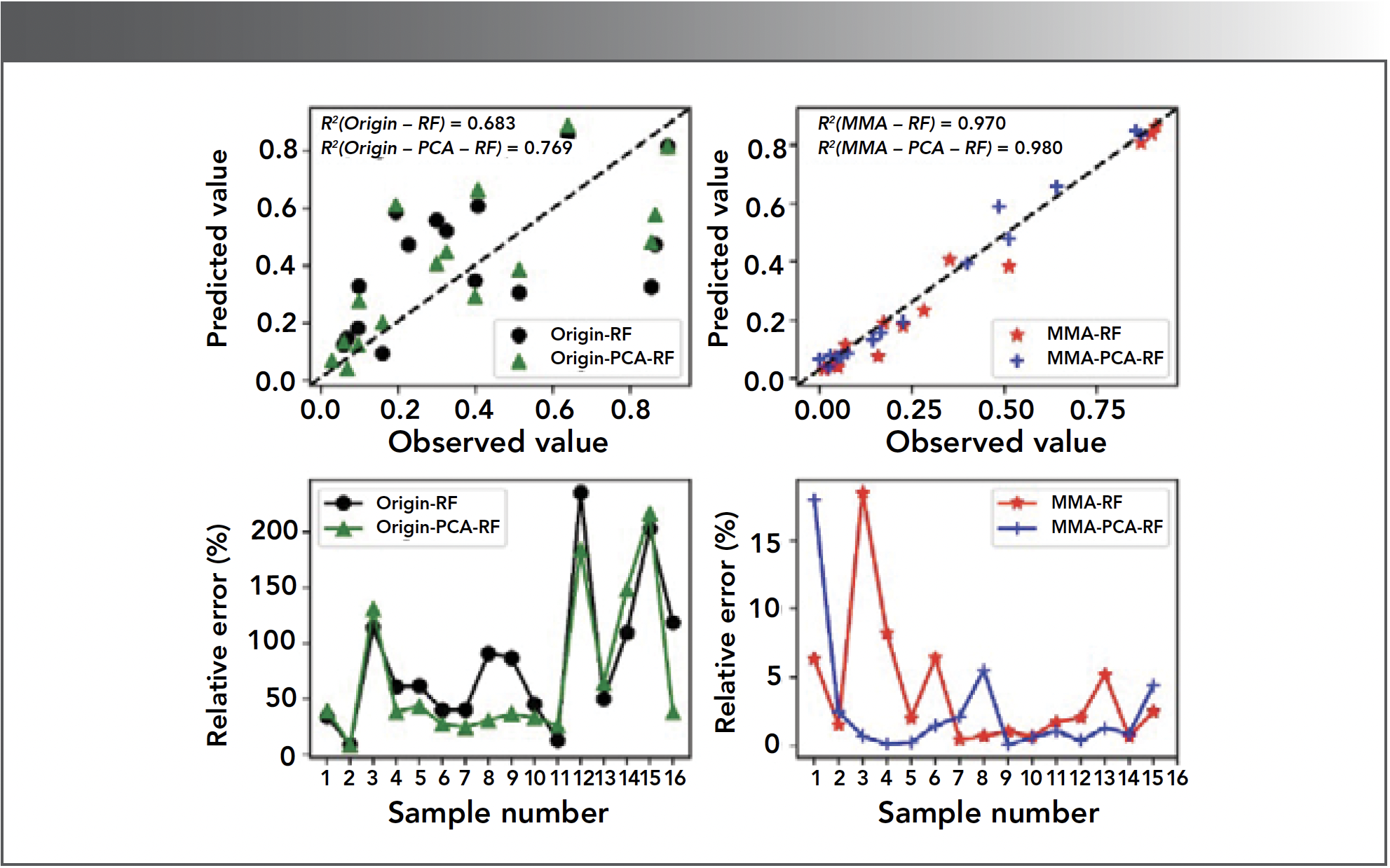
To more clearly illustrate the benefits of our method for modeling, we report the results from all the models in Table III. All of them are trained and evaluated on the same data set (the training set is 80%) with 100 repetitions. The result obtained by Bao and colleagues (7) (using wavelet decomposition and random forest method) are also listed in Table III as a comparison. In addition, the observed and predicted values of SOM contents, together with the relative error obtained by the origin-based and MMA-based models coupling with RF, on the testing set are shown in Figure 7. Our findings concluded that:

• Compared to the models on the left side (without PCA), PCA processing on the right side brings better, higher R² and lower RMSE, no matter the training set or testing set.
• As expected, the MMA-based sensitive bands extraction method led to great model performance improvement. The determination coefficient (R²) increased by 42% and 47% (without PCA), 23% and 31% (with PCA processing), for RF and SVM methods, respectively for the testing set (the results are highlighted).
• Compared with Bao’s model, our model has obvious advantages on the testing set.
• When comparing the two intelligent regression algorithms, RF makes the models more accurate and stable.

FIGURE 7: Comparing the prediction effect between the origin-based and MMA-based models by using RF method. The upper two panels are the observed values versus to predicted values of the SOM contents (all the values are normalized; the black fold line denotes the line y = x). The bottom subplots are the relative error between the predicted and observed values.

In summary, the MMA-based sensitive bands extraction method can effectively help improve the performance of the SOM prediction model.

Conclusion

The soil hyperspectral reflects rich SOM information; however, it is awash with much redundancy, which interferes with the modeling for SOM content estimation. Therefore, finding the most significant reflection region (sensitive bands) in the spectral bands range is an important task before SOM modeling. In this paper, we calculated the local Hurst exponent by MMA and found several crossovers (the mutation points of fractal structure). According to the crossovers, we speculated that they might correspond to the sensitive bands. Correlation analysis between the SOM content and the local exponent confirmed our conjecture. Thus, we used this idea to determine the sensitive bands of the soil spectrum. After verification, the sensitive bands of all samples were located at approximately 359–405 nm. To further eliminate redundancy information in the sensitive bands, traditional PCA was employed for us. Unexpectedly, we found that the contribution of the first principal component reached 99.97%. Therefore, the first principal component of reflectivity in the sensitive bands was used as the input for modeling SOM estimation. Two intelligent regression algorithms of RF and SVM were used. As a comparison, the two algorithms were also used on the model input by the reflectivity of original bands and without PCA processing. The results show that the MMA method combined with the PCA could significantly improve the model performance. Among those models, the MMA-based models combined with RF are recommended for SOM estimation.

It is worth mentioning that the concept of sensitive band detection by the MMA proposed in this work can be applied in other fields, for example, crop nutrition diagnosis based on the hyperspectral features, cultivated land identification by using remote sensing signal, object detection by using radar signal, and so on.

Funding

Funding National Natural Science Foundation of China (61973111); the Key Foundation of Hunan Educational Committee (CN) (22A0135), Natural Science Foundation of Hunan Province (2023JJ30304); National Science and Technology Basic Work Special Project (2014FY110200).

Acknowledgments

The authors wish to thank the anonymous reviewers, as well as Jerome Workman Jr. and Laura Bush, for their constructive comments and suggestions, which led to a great improvement to the presentation of this work.

Disclosures

The authors declare no conflicts of interest.

References

(1) Guo, J.; Zhao, X.; Guo, X.; et al. Inversion of Organic Matter Content in Red Soil Based on PLSR-BP Composite Model. Acta Pedol. Sin. 2020, 57 (3), 636–645. DOI: 10.11766/trxb201904160060

(2) Thenkabail, P. S.; Lyon, J. G. Hyperspectral Remote Sensing of Vegetation; CRC Press, 2011.

(3) Tong, Q.; Zhang, B.; Zhang, L. Current Progress of Hyperspectral Remote Sensing in China. J. Remote Sens. 2016, 20 (5), 689–707. DOI: 10.11834/jrs.20166264

(4) Zhang, Z.; Lao, C.; Wang, H.; Karnieli, A.; Chen, J.; Li, Y. Estimation of Desert Soil Organic Matter through Hyperspectra Based on Fractional-Order Derivatives and SVMDA-RF. Trans. Chin. Soc. Agric. Mach. 2020, 51 (1), 156–167. DOI: 10.6041/j.issn.1000-1298.2020.01.017

(5) Zhu, Y.; Yu, L.; Hong, Y.; et al. Hyperspectral Features and Wavelength Variables Selection Methods of Soil Organic Matter. Sci. Agric. Sin. 2017, 50 (22), 4325–4337. DOI: 10.3864/j.issn.05781752.2017.22.009

(6) Wu, Y.; Zhou, Y.; Sheng, D.; Ye, X. Hyperspectral Band Selection Based on Optimal Linear Prediction of Principal Components in Subspace. J. Infrared Millimeter Waves 2018, 37 (1), 119–128. DOI: 10.11972/j.issn.1001-9014.2018.01.021

(7) Bao, Q.; Ding, J.; Wang, J.; Cai, L. Hyperspectral Detection of Soil Organic Matter Content Based on Random Forest Algorithm. Arid Land Geography 2019, 42 (6), 1404–1414. DOI: 10.12118/j.issn.1000-6060.2019.06.20

(8) Mandelbrot, B. B. A Multifractal Walk Down Wall Street. Sci. Am. 1999, 298, 70–73. DOI: 10.1038/scientificamerican0299-70

(9) Wang, X.; Wang, F.; Liao, G.; Guan, C. Multifractal Analysis of Rapeseed Spectrum for Chlorophyll Diagnosis Modeling. Spectrosc. Spec. Anal. 2016, 36 (11), 3657–3663. DOI: 10.3964/j.issn.1000-0593(2016)11-3657-07

(10) Jiang, S.; Wang, F.; Shen, L.; Liao, G.; Wang, L. Extracting Sensitive Spectrum Bands of Rapeseed Using Multiscale Multifractal Detrended Fluctuation Analysis. J. Appl. Phys. 2017, 121, 104702. DOI: 10.1063/1.4978308

(11) Jiang, S.; Wang, F.; Shen, L.; Liao, G. Local Detrended Fluctuation Analysis for Spectral Red-Edge Parameters Extraction. Nonlinear Dyn. 2018, 93, 995–1008. DOI: 10.1007/s11071-018-4241-y

(12) Qi, J.; Fan, F.; Guo, Z. Monitoring Tobacco Canopy Growth Status Based on Hyperspectral Fractal Analysis. J. South China Norm. Univ., Nat. Sci. Ed. 2016, 48 (1), 94–100. DOI: 10.6054/j.jscnun.2015.11.001

(13) Chávez, P.; Yarlequé, C.; Loayza, H.; et al. Detection of Bacterial Wilt Infection Caused by Ralstonia solanacearum in potato (Solanum tuberosum L.) Through Multifractal Analysis Applied to Remotely Sensed Data. Precis. Agric. 2012, 13 (2), 236–255. DOI: 10.1007/s11119-011-9242-5

(14) Wang, T.; Zhou, C.; Gu, Y.; Ma, W.; Liu, Y.; Wei, H. Hyperspectral Estimation of Cadmium Content in Tumorous Stem Mustard Based on the Wavelet-Fractal Analysis. Sci. Agric. Sin. 2018, 51 (1), 71–81. DOI: 10.3864/j.issn.0578-1752.2018.01.007

(15) Liu, F.; Wang, F.; Liao, G.; Lu, X. Prediction of Oleic Acid Content of Rapeseed Using Hyperspectral Technique. Appl. Sci. 2021, 11 (12), 5726. DOI: 10.3390/app11125726

(16) Peng, C. K.; Buldyrev, S. V.; Havlin, S.; Simons, M.; Goldberger, A. L. Mosaic Organization of DNA Nucleotides. Phys. Rev. E 1994, 49, 1685–1689. DOI: 10.1103/PhysRevE.49.1685

(17) Kantelhardt, J. W.; Zschiegner, S. A.; Koscielny-Bunde, E.; Havlin, S.; Bunde, A.; Stanley, H. E. Multifractal Detrended Fluctuation Analysis of Nonstationary Time Series. Phys. A (Amsterdam, Neth.) 2002, 316 (1–4), 87–114. DOI: 10.1016/S0378-4371(02)01383-3

(18) Zhang, X.; Liu, H.; Zhao, Y.; Zhang, X. Multifractal Detrended Fluctuation Analysis on Air Traffic Flow Time Series: A Single Airport Case. Phys. A (Amsterdam, Neth.) 2019, 531, 121790. DOI: 10.1016/j.physa.2019.121790

(19) Pavlov, A. N.; Runnova, A. E.; Maksimenko, V. A.; Pavlova, O. N.; Grishina, D. S.; Hramov, A. E. Detrended Fluctuation Analysis of EEG Patterns Associated with Real and Imaginary Arm Movements. Phys. A (Amsterdam, Neth.) 2018, 509, 777–782. DOI: 10.1016/j.physa.2018.06.096

(20) Jiang, Z.; Xie, W.; Zhou, W.; et al. Multifractal Analysis of Financial Markets: A Review. Rep. Prog. Phys. 2019, 82 (12), 2349. DOI: 10.1088/1361-6633/ab42fb

(21) Wang, F.; Liao, D.; Li, J.; Liao, G. Two-Dimensional Multifractal Detrended Fluctuation Analysis for Plant Identification. Plant Methods 2015, 11, 12. DOI: 10.1186/s13007-015-0049-7

(22) Wang, F.; Li, Z.; Li, J. Local Multifractal Detrended Fluctuation Analysis for Non-Stationary Image’s Texture Segmentation. Appl. Surf. Sci. 2014, 233, 116–125. DOI: 10.1016/j.apsusc.2014.10.065

(23) Wang, F.; Wang, L.; Chen, Y. A DFA-Based Bivariate Regression Model for Estimating the Dependence of PM2.5 Among Neighbouring Cities. Sci. Rep. 2018, 8, 74–75. DOI: 10.1038/s41598-018-25822-w

(24) Gieraltowski, J.; Zebrowski, J. J.; Baranowski, R. Multiscale Multifractal Analysis of Heart Rate Variability Recordings with a Large Number of Occurrences of Arrhythmia. Phys. Rev. E 2012, 85 (1–2), 021915. DOI: 10.1103/physreve.85.021915

(25) Gieraltowski, J.; Hoyer, D.; Tetschke, F.; Nowack, S.; Schneider, U.; Zebrowski, J. Development of Multiscale Complexity and Multifractality of Fetal Heart Rate Variability. Auton. Neurosci. 2013, 178 (1–2), 29–36. DOI: 10.1016/j.autneu.2013.01.009

(26) Fan, Q.; Liu, S.; Wang, K. Multiscale Multifractal Detrended Fluctuation Analysis of Multivariate Time Series. Phys. A (Amsterdam, Neth.) 2019, 532, 121864. DOI: 10.1016/j.physa.2019.121864

(27) Lin, A.; Ma, H.; Shang, P. The Scaling Properties of Stock Markets Based on Modified Multiscale Multifractal Detrended Fluctuation Analysis. Phys. A (Amsterdam, Neth.) 2015, 436, 525–537. DOI: 10.1016/j.physa.2015.05.041

(28) Fan, Q. Asymmetric Multiscale Detrended Fluctuation Analysis of California Electricity Spot Price. Phys. A (Amsterdam, Neth.) 2016, 442, 252–260. DOI: 10.1016/j.physa.2015.08.056

(29) Wang, J.; Shang, P.; Cui, X. Multiscale Multifractal Analysis of Traffic Signals to Uncover Richer Structures. Phys. Rev. E 2014, 89, 032916. DOI: 10.1103/PhysRevE.89.032916

(30) Wang, F.; Fan, Q.; Stanley, H. E. Multiscale Multifractal Detrended-Fluctuation Analysis of Two-Dimensional Surfaces. Phys. Rev. E 2016, 93, 042213. DOI: 10.1103/PhysRevE.93.042213

(31) Ge, E.; Leung, Y. Detection of Crossover Time Scales in Multifractal Detrended Fluctuation Analysis. J. Geogr. Syst. 2013, 15 (2), 115–147. DOI: 10.1007/s10109-012-0169-9

(32) Dong, F., Data Analysis Mining and Visualization Using Python; Posts & Telecom Press, 2020.

(33) Hu, P.; Chen, Y.; Jiang, C.; et al. Spectral Observation and Classification of Typical Tree Species Leaves Based on Indoor Hyperspectral Lidar. J. Infrared Millimeter Waves 2020, 39 (3), 372–380. DOI: 10.11972/j.issn.1001-9014.2020.03.016

Shaofang He, Luming Shen, and Jing Yang are with the College of Information and Intelligence at Hunan Agricultural University, in Changsha, China. Fang Wang is with the Key Laboratory of Intelligent Computing and Information Processing of Ministry of Education and Hunan Key Laboratory for Computation and Simulation in Science and Engineering at Xiangtan University, in Xiangtan, China. Qing Zhou is with the College of Resources and Environment at Hunan Agricultural University, in Changsha, China. Direct correspondence to: popwang619@163.com