Addendum to Chemometrics in Spectroscopy
This column is the continuation of a series (1-5) dealing with the rigorous derivation of the expressions relating the effect of instrument (and other) noise to its effects on the spectra we observe. Our first column in this series was an overview. While subsequent columns dealt with other types of noise sources, the ones listed analyzed the effect of noise on spectra when the noise is constant detector noise (that is, noise that is independent of the strength of the optical signal). Inasmuch as we are dealing with a continuous series of columns, on this branch in the thread of the discussion, we again continue the equation numbering and use of symbols as though there were no break. The immediately previous column (5) was the first part of this set of updates of the original columns.


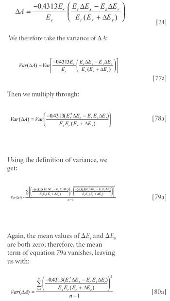
Here we pick up from where we left off. Figure 1a shows what happens to the noise level, for the same condition of constant "sample transmittance" as a function of signal-to-noise ratio (S/N), for different values of sample transmittance. In the "low noise" regime, the noise has the behavior we have derived for it. However, the effect of the exaggeration of the random variations very quickly takes over, and in the "high noise" regime there is virtually no difference in the noise behavior at different values of transmittance because that is now dominated by the divergence of the integrals involved.


Jerome Workman, Jr.
A verification of the effects seen in Figure 1 is presented in Figure 2, in which we present a graph showing the transmittance noise as a function of the sample transmittance (Es/Er). Except for the occasional spike, when S/N is 5 and even when it is only 4.5, the transmittance noise varies essentially, as we saw in working out the exact solution for transmittance noise in the low-noise case. Naturally, the underlying transmittance noise value is higher when the reference S/N is lower. When S/N decreases to 4, "spikes" happen frequently enough that it becomes almost impossible to tell where the "underlying" transmittance noise level is, because the computed values are again dominated by the divergent integrals.


Howard Mark
Absorbance Noise in the "High Noise" Regime
Just as equation 5, which led to equation 76a, was the starting point for investigating the behavior of transmittance noise in the high noise regime, so too is equation 24 the starting point for investigating the behavior of absorbance noise in the high noise regime. While we presented equation 24 previously, in the original analysis, we did not follow through to investigate its behavior, because we went directly to the analysis of the behavior of Var (ΔA/A), instead. Therefore, we present equation 24 again and take this opportunity to investigate it:


Again we see that the variance of the absorbance equals (n - 1)/n times the mean value of the summand of equation 80a, and also that we can ignore the premultiplier term (n - 1)/n for large values of n.


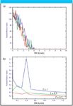
Figure 1: (a) Transmittance noise as a function of reference S/N, at various values of sample transmittance. (b) Expansion of Figure 1a.
We begin our investigation of the behavior of the absorbance noise by comparing it to the theoretical expectation from the low-noise condition according to equation 32 (3). This comparison is shown in Figures 3a and 3b. These figures show what we might expect: that as S/N increases, the computed value approaches the theoretical value for the low-noise approximation, and also an excessive bulge at very low values of S/N, apparently similar to the abnormally large values observed in the behavior of the transmittance at very low values of S/N. After performing this comparison, we will not pursue the analysis any further, as we will obtain the results we would expect to get from the analysis of the transmission behavior.


Figure 2: Transmittance noise as a function of transmittance, for different values of reference energy S/N (recall that, since the standard deviation of the noise equals unity, the set value of the reference energy equals S/N).
There is, however, something unexpected about Figure 3a. That is, the decrease in absorbance noise at the very lowest values of S/N (those lower than approximately Er = 1). This decrease is not a glitch or an artifact or a result of the random effects of divergence of the integral of the data such as those we saw when performing a similar computation on the simulated transmission values. The effect is consistent and reproducible. In fact, it appears to be somewhat similar in character to the decrease in computed transmittance we observed at very low values of S/N for the low-noise case.


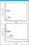
Figure 3: (a) Comparison of computed absorbance noise to theoretical value for the low-noise case (according to equation 32), as a function of S/N, for constant transmittance (set to unity). (b) Expansion of Figure 3a.
Jerome Workman, Jr. serves on the Editorial Advisory Board of Spectroscopy and is director of research and technology for the Molecular Spectroscopy & Microanalysis division of Thermo Fisher Scientific. He can be reached by e-mail at: jerry.workman@thermo.com.
Howard Mark serves on the Editorial Advisory Board of Spectroscopy and runs a consulting service, Mark Electronics (Suffern, NY). He can be reached via e-mail: hlmark@prodigy.net.
References
(1) H. Mark and J. Workman, Spectroscopy 15(10), 24–25 (2000).
(2) H. Mark and J. Workman, Spectroscopy 15(11), 20–23 (2000).
(3) H. Mark and J. Workman, Spectroscopy 15(12), 14–17 (2000).
(4) H. Mark and J. Workman, Spectroscopy 16(2), 44–52 (2001).
(5) H. Mark and J. Workman, Spectroscopy 22(5), 14–21 (2007).


LIBS Illuminates the Hidden Health Risks of Indoor Welding and Soldering
April 23rd 2025A new dual-spectroscopy approach reveals real-time pollution threats in indoor workspaces. Chinese researchers have pioneered the use of laser-induced breakdown spectroscopy (LIBS) and aerosol mass spectrometry to uncover and monitor harmful heavy metal and dust emissions from soldering and welding in real-time. These complementary tools offer a fast, accurate means to evaluate air quality threats in industrial and indoor environments—where people spend most of their time.

Smarter Sensors, Cleaner Earth Using AI and IoT for Pollution Monitoring
April 22nd 2025A global research team has detailed how smart sensors, artificial intelligence (AI), machine learning, and Internet of Things (IoT) technologies are transforming the detection and management of environmental pollutants. Their comprehensive review highlights how spectroscopy and sensor networks are now key tools in real-time pollution tracking.

New AI Strategy for Mycotoxin Detection in Cereal Grains
April 21st 2025Researchers from Jiangsu University and Zhejiang University of Water Resources and Electric Power have developed a transfer learning approach that significantly enhances the accuracy and adaptability of NIR spectroscopy models for detecting mycotoxins in cereals.


