What Can NIR Predict?
Columnists Howard Mark and Jerome Workman, Jr. discuss the application of chemometric methods of relating measured NIR absorbances to compositional variables of samples.

In more recent times, great interest has been shown, and much energy expended, on calibration transfer: the ability to create a quantitative calibration model from data measured on one instrument and use that model to predict samples measured by a different instrument. An equivalent although not identical concept, used in the early days of near-infrared (NIR) spectroscopy, was "universal calibration": creation of a single model from data measured on two or more instruments that could then be used for predicting the composition of samples measured on any of those instruments.

Jerome Workman, Jr.
For either of these approaches to be successful, it obviously is necessary that the instruments be able to give the same predicted values for the same samples when using the same calibration model, regardless of the nature of the model. Recently, some data have become available that allow for some interesting tests of this concept. The data were described by Ritchie and colleagues (1). It is available on-line, along with a description, at http://www.idrc-chambersburg.org/shootout_2002.htm. The availability of this data led to thoughts of performing a computer experiment to examine the behavior of the way various calibration models would interact with the data.

Howard Mark
The data consist of NIR absorbance readings, measured on two instruments, arbitrarily designated 1 and 2, of a set of pharmaceutical tablets. Although not mentioned in the original publication (1), for a sample from a given lot, the same tablet was used for the measurement on both instruments. The only difference between measurements was that the tablet was oriented randomly with the embossed face up or down, between instruments, the intention being to present the various lots of tablets to the instrument in "random" orientation so that orientation effects would be minimized (2).
The calibration sets contained data from 155 tablets, and because of the initial purpose for collecting the data, covered a fairly broad range of values for the analyte: from roughly 150 mg to almost 250 mg of analyte per tablet. Validation sets of data also were available, although they did not include as broad a range of analyte. One validation set (here called validation set 1) contained 40 spectra (again, from the same samples measured on each instrument); the other (called the "test" set in the original data set but which we here call validation set 2) contained 460 samples. All spectra had corresponding values for the analyte, measured by the reference laboratory using the appropriate validated method. The data have been organized so that the samples were present in the same order in corresponding members of each pair of datasets.
Results from a Model Created Using Real Reference Values
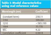
The calibration results we will use, computed using the reference values provided with the data and the spectroscopic absorbance values from the calibration data set measured on instrument 1, are given in Table I. The results we develop here differ from the published results (1) for several reasons:
- Here we used multiple linear regression (MLR) to create the calibration models, whereas the published results used principal component regression (PCR) and partial least squares (PLS) to create the calibration models. PLS and PCR calibration models are expected to behave similarly to what we found here (see the following).
- No attempt was made here to optimize the data transforms or other characteristics of the model; also, no "outliers" were removed. Indeed, no modifications of any type were made to the measured data.
The model obtained, and its performance characteristics, are presented in Table I.

Table I: Model characteristics using real reference values
The prediction performance of the model for the six data sets available is presented in Table II. No changes, modifications, or transforms were applied to any of the data, nor was the model modified in any way before using it for prediction of any of the other sets. Also, no bias correction or other modification was made to the predicted values used to calculate the standard error prediction (SEP).

Table II: (SEE)/SEP
We note a moderate increase in the error for instrument 2, compared with instrument 1, for all three data sets. This is likely caused by a small bias in the predictions from instrument 2. Arguably, the standard error of the estimate (SEE) for instrument 1 should not be compared with the SEPs for all the other cases, but because it bears the same relationship to the corresponding results from instrument 2 for the same data set as the other data sets do, this result seems satisfactory. The point of the exercise here is not simply to obtain a "best" calibration, or even to demonstrate transferability per se.
The point of the exercise is to determine the degree of agreement between the values predicted by the model, on the data from the two instruments. For this purpose, we calculate the standard deviation of the differences between the predicted values from the two instruments on the same samples, using the formula:

where:
Xj1, Xj2 represent the data from the jth sample measured on instruments 1 and 2, respectively.
n is the number of samples.
We also computed the correlation coefficient between the predicted values from the two corresponding data sets (this is an exception to the rule of not modifying the data in any way, but mean-subtraction was applied to the two data sets of necessity because it was an inherent part of the calculation of correlation coefficient); the two statistics for the relationship between each pair of data sets are presented in Table III, for further reference.

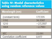
Table IV: Model characteristics using random reference values
It is particularly noteworthy that the correlation coefficient between the predictions (0.9897) for the calibration data set is higher between the values from the two instruments than for the single instrument against the reference values (0.9818).
We present a comparative plot of the prediction results from the two instruments in Figure 1; each part of Figure 1 shows the results from one of the three data sets used. The other two plots are similar.
Results from a Model Created Using Random Reference Values
Now comes the really interesting stuff. The exercise was repeated after the reference values were replaced by random numbers. The MATLAB random function was used to create a set of normally distributed quasi-random values. A constant was then added to each value, and then the set of random numbers was scaled so that the mean and standard deviation of the random numbers matched the corresponding statistics of the reference values used for the original calibration.

Table V: Standard deviation of differences between instruments for random calibration values
Again, the MLR calibration algorithm was used, and the same wavelengths used for the original model were used to create the model against the random "reference data." No change or modification was made to either the data or the model before using them for the predictions. Table IV presents the characteristics of the model arrived at.

Figure 1: Values predicted from the two instruments, using the model from Table I, created using real reference values: (a) Comparing instruments (a) using calibration data sets, (b) using the first pair of validation data sets, and (c) using the second pair of validation data sets.
Not surprisingly, the model performs poorly compared to the model for real reference values. The standard error of the calibration (SEC) is much larger than when the calibration was performed against real data with similar characteristics, and the correlation with the random numbers is virtually zero. This last point also is hardly surprising.
Given that the calibration results are so poor, we forbear to calculate the SEPs for the various other data sets: the calibration set run on the second instrument, or the two validation sets run on the two instruments. The prediction performance will not be any better; we will see the reason for this a little further on.
Much more interesting, and pertinent, is what we find when we redo the calculations for comparing the results from the two instruments. These are presented in Table V, which should be compared with Table III.
We finish our presentation of the calibration and prediction results by plotting the predicted values from the two instruments, for each corresponding pair of predictions, just as we did for the first round of calculations (based upon calibrations against real reference values). These plots are shown in Figure 2.

Figure 2: Values predicted from the two instruments, using the model from Table IV, created using random reference values: Comparing instruments (a) using calibration data sets, (b) using the first pair of validation data sets, and (c) using the second pair of validation data sets.
What we find in Table V is that not only are the prediction results obtained from comparing the two instruments much better than when comparing the predicted values against the reference values, they are also much better than the results obtained when a "real" calibration was used.
So What Does It All Mean?
We will make some predictions, although we refuse to estimate an SEP for the predictions despite the fact that in our own heads, we put the probability at well over 90% that we're going to get a lot of flak over this. However, all we did was to do a computer experiment, and merely presented the results.
Our first prediction is that the more outraged segment of the readership will accuse us of "proving" something like "NIR doesn't work," or something equally silly, but that accusation is nonsense. First of all, NIR does work, as we all know and as proven by over 30 years of successful usage. Indeed, as we will show below, these results occur only because NIR works, and works very well. If NIR didn't work, the interinstrument agreement would be very poor indeed, at least as poorly as the NIR calibrations agreed with the random data.
Moreover, a moment's thought would reveal to even the most casual reader that if in fact we could "prove" that "NIR doesn't work," then we certainly wouldn't do it, since we work in NIR and that's how we earn a living. Or do our readers think that we're really so insane as to kill the goose that's laying the golden eggs for our colleagues and ourselves? Obviously not.
Our second prediction is that a less outraged (but perhaps somewhat more pleased) segment of the readership will enjoy the fact that they will think that we've "proved" something like "MLR doesn't work." This segment of the readership has an interest in avoiding and denigrating the use of MLR in favor of promoting the full spectral calibration methods: PCR and PLS. But an accusation like that is also nonsense, for the same reasons given earlier about NIR itself. Furthermore, what makes anyone think that PCR or PLS calibrations are immune from similar behavior? In fact, they are not safe from these effects; We're fully convinced that if PCR or PLS were used to create the calibration models and the same exercise was performed for the rest of the calculations, they would obtain the same, or at least equivalent, results. And the proponents of these full-spectrum methods should be glad of that, because the fact that such results are obtained is also due to the twin facts that PLS and PCR work as well as MLR and NIR itself do.
So what, in fact, did we demonstrate with this little computer experiment? What we showed was that if the spectra are good, and the sample set is robust and adequate to support a calibration, then NIR agrees with NIR, whether or not it agrees with anything else. In fact, we can see that the agreement between the two instruments was considerably better than the agreement with the reference laboratory, regardless of which model was used.
One point of fact is not obvious from this discussion, however. The agreement between instruments is real, although somewhat nebulous, because an examination of the range of values the predictions for the random values cover is much smaller than the original range of the reference data, despite the fact that the random values used for calibration were adjusted to have the same statistics. An examination of the various scatter plots in Figure 2 shows that the range of predicted values is 5–10 units, as compared with the roughly 100 unit range seen in Figure 1, and as represented in the reference laboratory values. To this extent, the smaller value of the SDdiff seen in Table V is not commensurate with the SDdiff in Table III. The correlation coefficients, however, being dimensionless quantities, are comparable.
The explanation of all of this is as follows: the samples comprising all the data sets involved exhibit real spectral differences between the various tablets making up the set. These spectral differences are systematic, and not random. In fact, this is what is meant by the phrase we used previously, that NIR "works"; now we see that in fact, that phrase is just a shorthand way to say that the compositions of samples in a set affect the measured spectra in a systematic way, so that a calibration model, if properly generated, will convert those spectral changes to compositional information in a correspondingly systematic manner.
Because the spectral absorbances are inherent properties of the samples, the measured spectra have the same relationships to each other regardless of the instrument on which they are measured, as long as the instruments themselves are proper ones for making the measurements in the first place. Therefore, when you multiply the spectra by the coefficients of a calibration model, the spectral differences create systematic effects on the predicted values, and these effects are the same on the different instruments. Therefore, it matters not what the calibration models represent, as long as they respond to the systematic changes in the spectra and not to any underlying random (that is, noise) content of those spectra.
As we have seen, this phenomenon is exactly what we found in the computer exercises we performed and reported above. The coefficients of the models are merely multipliers of the systematic effects present in the underlying spectral data. Because those are the same in both instruments, then of course the predicted values agree between the two instruments and give a very high correlation between the instruments' predicted values.
This also explains why the instruments agree better with each other than with the reference laboratory values. The instruments are using only the systematic variations of the underlying spectra, not the reference laboratory values, in making the predictions or the comparisons. Therefore, the reference laboratory error, which is an independent random phenomenon, is rejected from the comparison and cannot influence it.
This situation can break down, however, under certain circumstances. A requirement of most concern is that the calibration model used, regardless of its origin, must be sensitive to the underlying spectral changes and be unaffected by the random (noise) content of the spectra. This, of course, is and always has been the hallmark of "good" calibration models. However, it always has been difficult to determine when that property existed in a model. Most attempts at developing criteria for making that determination have been based upon comparisons between the instrument and reference laboratory results, thereby introducing the reference laboratory error into the calculation and creating an unnecessarily high barrier to "seeing" through the noise.
The most common way that the benefits of the interinstrument comparisons can be lost is if the model becomes more sensitive to the noise content of the spectra than necessary. This is another way to describe the term (somewhat loosely) thrown around: "overfitting." One of the consequences of overfitting is inflation of the magnitudes of the calibration coefficients; this is the underlying cause of increased sensitivity to noise (see pages 55–56 in reference 3). It seems likely that this new method of comparing instrument predictions will be more sensitive to the effect of overfitting, since there is not (constant, and larger) reference value error to overwhelm it.
By removing the reference laboratory errors from the comparison, we've seen that the underlying agreement between instruments is a necessary result of the expression of the underlying spectral behavior of the samples and of their relative compositions. This all has several consequences:
- It further demonstrates the need for superior reference laboratory values to obtain a model that will accurately predict future samples (as though any of us needed further proof of that!).
- Reference laboratory results for an NIR calibration should never, ever be obtained from another NIR instrument since we can expect that the NIR instrument we are calibrating will agree with that other NIR instrument whether or not either one agrees with reality. Even if the NIR "reference" values are valid, the diagnostic statistical evaluations of the model will be excessively and misleadingly optimistic because, as we have seen, the inter-instrument agreement is smaller than the "true" SEP.
- The model we use will key on to the real, underlying spectral variations in the samples, as expressed in the measured spectra. This is the reason the two instruments agreed so well, regardless of the model used.
- As a consequence of the third point, the agreement between instruments is another way that "overfitting" can be detected. When the model becomes more sensitive to the noise of the measurement than to the actual spectral changes, the agreement between the instruments can be expected to break down, and this will indicate that overfitting is occurring. Because the reference laboratory values themselves are not involved in the comparison, the error of the reference laboratory will not affect the comparison. Furthermore, since the error of the reference laboratory values is usually larger than that of the NIR measurement, comparison of two instruments in this manner provides a more sensitive method of detecting any overfitting that might occur.
- By virtue of the agreement between instruments being due solely to the effects of the underlying spectral changes in the samples, this constitutes a "proof" that NIR works. Secondarily, it provides a "proof" that MLR works. We leave the "proof" that PCR and PLS "work" to those with interest in such things. These data are available online as described above.
- Going back to the starting point of this column, agreement between instruments is a necessary condition for calibration transfer. It is not a sufficient condition, however, because if one instrument predicts the analyte of interest poorly, then another instrument can be expected to perform equally poorly, at best (refer to the second point, earlier, for a reminder of the reason for this). Nevertheless, the potential to transfer calibrations can be demonstrated independently of having an actual calibration to transfer. The ability to actually transfer a calibration, however, will depend, as it does now, upon the particular calibration as well as on the instruments being used. Nevertheless, direct comparison of predictions from the two instruments in the manner shown here provides another tool in the toolbox for evaluating the situation.
- Since even random calibration data do not disrupt the agreement due to systematic effects in the spectra, this approach is another way to detect "overfitting" even on a single instrument. It is common practice nowadays to measure multiple spectra from the calibration samples. This being the case, the different readings can be separated into subsets, each subset containing one of the spectra from each sample. Then, after a calibration is developed, the agreement between the various subsets can be calculated (for example, by the standard deviation from each sample, with all these standard deviations pooled over the sample set). If this is done for a varying number of factors, and for different data transformations, it will quickly become apparent when the contribution of the instrumental variations and effect of the model make appreciable contributions to the total error.
It is interesting to consider the phenomena that can cause the correlation between instruments to break down:
- Excess noise of the instrument. It is noteworthy that the spectra used, having been measured by transmission through a tablet, had absorbances as high as six absorbance units, although the wavelengths used for the MLR calibrations obtained here had absorbances of "only" 3.5–5 absorbance units. Nevertheless, the superior results for the interinstrument comparisons were obtained. This is testimony to the quality of modern NIR instruments, but more importantly, it shows that when good samples are available, good results can be obtained despite conditions being such that we would expect the noise to dominate. We note parenthetically here that an absorbance value of 3 corresponds to measuring only 0.1% of the original spectral signal; thus S/N is decreased by roughly 1000-fold.
And we still obtained such good results — NIR really must work, mustn't it?
- As described earlier, we expect that overfitting will be a factor causing problems in this respect, through the mechanism of inflating the calibration coefficients.
- "Sample noise." We coin this term here to represent the effect of the differences between repacks, different particle size samples, and the effects of other such phenomena on the readings, which often cannot be taken into account completely by the model. Because the particle size effect is random from sample to sample, we can expect that this will cause an extraneous random effect on the predicted values. In the current experiment, the tablets would not have a random effect of this nature since each tablet is fixed and reproducible, and the same tablet was presented to both instruments. Samples composed of packed powders, however, are liable to be affected by this.
Jerome Workman, Jr. serves on the Editorial Advisory Board of Spectroscopy and is director of research and technology for the Molecular Spectroscopy & Microanalysis division of Thermo Fisher Scientific. He can be reached by e-mail at: jerry.workman@thermo.com
Howard Mark serves on the Editorial Advisory Board of Spectroscopy and runs a consulting service, Mark Electronics (Suffern, NY). He can be reached via e-mail: hlmark@prodigy.net
Note
We would appreciate hearing from anyone who repeats this exercise using PCR or PLS or any other full-spectrum calibration method. Please let us know your results.
References
(1) G.E. Ritchie, R.W. Roller, E.W. Ciurczak, H. Mark, C. Tso, and S.A. Macdonald, J. Pharm. Biomed. Anal.29(1-2), 159–171 (2002).
(2) G. Ritchie, private communication (2006).
(3) H. Mark, Principles and Practice of Spectroscopic Calibration (John Wiley & Sons, Inc., New York, 1991).

From Classical Regression to AI and Beyond: The Chronicles of Calibration in Spectroscopy: Part I
February 14th 2025This “Chemometrics in Spectroscopy” column traces the historical and technical development of these methods, emphasizing their application in calibrating spectrophotometers for predicting measured sample chemical or physical properties—particularly in near-infrared (NIR), infrared (IR), Raman, and atomic spectroscopy—and explores how AI and deep learning are reshaping the spectroscopic landscape.