Classical Least Squares, Part V: Experimental Results

This column is the next continuation of our discussion of the classical least squares (CLS) approach to calibration (1–4). As we usually do, when we continue the discussion of a topic through more than one column, we continue the numbering of equations from where we left off.

In this column, we will be dealing largely with figures and the spectra therein. Having developed the theory behind CLS, the first question coming to our mind is, or should be, "How well does the theory work?" Can we in fact fit spectra of pure materials to a set of mixture spectra and from that, calculate via least squares methods (outlined in the previous column) the contributions of the spectra of the individual components to the spectra of the mixtures?

If in fact we can do that exercise correctly, then we should be able to reproduce the spectra of the mixtures. How can we reproduce the spectra of the mixtures? The answer is, "the same way we predict the concentrations of unknowns in a mixture when we use multiple linear regression (MLR) calibration methodology."

After all, when we calibrate a set of spectra for the concentrations of the components using MLR, we use least-squares calculations to determine the coefficients of the various wavelengths that, when multiplied by the spectra at the appropriate wavelengths, gives us the predicted values of the components.

Similarly, when we calibrate a set of pure-component spectra (as described in the previous column) against the spectrum of the mixture using CLS, we use least-squares calculations to determine the coefficients of the pure spectra that, when multiplied by the spectra (at all wavelengths), gives us the predicted values of the spectral contribution of that component to the mixture spectrum.

Note the parallel constructions of the descriptions of the CLS calculation and the MLR calculation. This parallel construction of the descriptions mirrors the parallel operations of the actual algorithms. Thus, in MLR we calibrate spectra against component concentrations, and then predict those component concentrations. Correspondingly, in CLS we calibrate spectra against other spectra (the spectra of mixtures) and then predict those mixture spectra.

Therefore, the bulk of this column will be graphical, oriented toward our visual evaluation of the spectra involved, and ultimately, comparing the predicted mixture spectra against the actual mixture spectra.

Experimental

We begin by describing how the data were developed, the experimental aspects. You don't think that we actually measured the spectra ourselves, do you? We've done that from time to time, but not in this case, because having been away from the lab for too long, and not having easily available facilities, it was best to have the spectra measured by someone who does this routinely. So the spectral data were actually collected by our good friend and colleague Ron Rubinovitz, at Buchi, Inc. (New Castle, Delaware). Of course, he used one of their own FT-NIR instruments, so the X-scale data, in contrast to much NIR data (where the wavelengths are measured in nanometers), were measured and are presented in wavenumbers, with units of waves per centimeter (or, as most descriptions of Fourier-transform techniques do, we could ignore the "waves" part and simply describe the units as 1/cm or cm^-1).

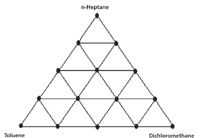
Figure 1: Graphical presentation of the three-component experimental mixture design.

The samples were made up by weight, as mixtures of the three materials described above: toluene, dichloromethane (CH₂Cl₂), and n-heptane. The target compositions were defined by a three-component mixture diagram, Figure 1 shows a graphical presentation of this experimental design, a presentation that allows us to see the relationships of the various mixtures. This design is the same one previously used to make up the water–methanol–acetic acid mixtures. It is unfortunate that those materials we previously used were unsuitable for the purpose we wanted them for here; nevertheless the design itself is robust and eminently suited to what we are trying to do. The design is symmetric and all components of the mixtures vary between 0% and 100% by weight. We also present the target numerical composition values of the samples comprising the mixture design in Table I. In this presentation, we can see that for all materials, the variations in composition of each component vary in increments of 25%, over the entire range of composition.

Table I: The values of the three components (in percent) for the 15 samples in the mixture design

All samples were measured using a 2-mm-thickness sample cuvette. The spectra were measured while the cuvettes were placed in a thermostated cuvette holder maintained at 35 °C to prevent spectral variations due to differences in temperature.

The experimental parameters are described in Table II.

Table II: Experimental conditions used

The Data

We start our description of the data with the spectra of the three clear liquids, representing the three pure materials that are all mutually completely miscible in all proportions. As we described in the previous columns in this subseries, we selected toluene, dichloromethane, and n-heptane as the materials to use to make our mixtures.

We will start by looking at the spectra of the pure materials that we are starting with. The transmission spectra (indicated by T) of these three materials are shown in Figure 2, both together (see Figure 2a) and separately (see Figures 2b–2d).

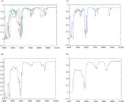
Figure 2: (a) Spectra of the pure components of our mixtures: toluene (blue), dichloromethane (green), and n-heptane (red). Spectra of pure (b) toluene, (c) dichloromethane, and (d) n-heptane.

We note from Figure 2 some features of these spectra. The first is that for all three materials, despite their chemical differences, the bands of all three materials fall into a few well-defined regions: 4000–5000 cm^-1 , 5000–6500 cm^-1 , 6500–7500 cm^-1 , and 7500–9000 cm^-1 .

For increased clarity, Figure 3 shows the expanded spectra of the three pure materials by spectral region. The need for the extra clarity will be obvious when we start to look more closely at the spectra of the mixtures: Figures 3a, 3b, 3c, and 3d present the 4000–5000 cm^-1 , 5000–6500 cm^-1 , 6500–7500 cm^-1 , and 7500–9000 cm^-1 regions expanded, respectively.

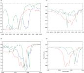
Figure 3: Spectra of pure components, by spectral region: (a) 4000–5000 cm-1 spectral region expanded, (b) 5000–6500 cm-1 spectral region expanded, (c) 6500–7500 cm-1 spectral region expanded, and (d) 7500–9000 cm-1 spectral region expanded. In all parts of this figure, toluene = blue, dichloromethane = green, n-heptane = red.

We note parenthetically that Figures 2a and 3a confirm our previous observation about the 4000–5000 cm^-1 spectral region, specifically that only in the 4000–4500 cm^-1 region is the absorbance so strong that the spectral curve "bottoms out."

To evaluate reproducibility of the measurements, in the face of possible composition changes due to differential evaporation of the mixture components while their spectra were measured, mixture samples were measured three times. Figure 4 presents the spectra for some of these mixtures. Mixtures of toluene and dichloromethane were selected for presentation in Figure 4a. These mixtures were chosen because toluene has the highest boiling point of the three components (110.3 °C) whereas dichloromethane has the lowest boiling point of the three (40.1 °C). These also represent the concentration extremes of any of the mixtures. Therefore, these samples represent the extremes of both boiling point and composition so that they would be most sensitive to any factors that caused any changes in the samples, and thus any differential evaporation, for example, would most likely show up in the mixtures of these materials.

Figure 4: Spectra of multiple repeat readings of several mixtures: (a) Mixture of 25% toluene, 75% dichloromethane, and (b) mixture of 75% toluene, 25% dichloromethane.

Each plot in Figure 4 represents triplicate readings of the indicated sample. Only one spectrum appears, because the spectra are so similar that they completely and exactly overlap each other, thus the spectrum from one reading hides the spectrum of each of the other two. This observation is important since it is our first indication that the mixtures are stable, as is the measurement of their spectra.

Examination of Figures 2a and 3a reveals a problem area in the spectra: The absorbance of all the components is so strong in the 4000–4500 cm^-1 spectral region that the spectra are clipped or flat-topped at T = 0.

The next set of data spectra that we examine are the spectra of the mixtures, shown in Figure 5. Figure 5a shows the spectra of all the mixtures used in the experiment. This figure further confirms our observation that the spectral region from 4000–4500 cm^-1 is clipped, for most, if not all, the samples. While the range 4000–5000 cm^-1 appears to include essentially the same absorbance bands, careful perusal of Figure 4a reveals that only the region of 4000–4500 cm^-1 are in fact, so strong as to clip; the region of 4500–5000 cm^-1 has no stronger bands than the 5000–6500 cm^-1 does. Thus, this region should be eminently useful to us.

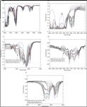
Figure 5: (a) Spectra of all mixtures, (b) spectra of all samples, in the spectral region 4000–5000 cm-1, (c) spectra of all samples, in the spectral region 5000–6500 cm-1, (d) spectra of all samples, in the spectral region 6500–7500 cm-1, and (e) spectra of all samples, in the spectral region 7800–9000 cm-1.

Figures 5b–5e present the spectra of all the mixtures in the various other spectral regions we have recognized above. A point of interest in these figures is that, as indicated by the marked sections of the figures, the experimental design used to create the set of mixtures is reflected in the absorbances of the mixtures in the various spectral regions indicated. While the component of the mixture corresponding to the indicated characteristics varies depending on the spectral region, we can note that in each of the spectral regions a single spectrum corresponds to the lowest transmission spectrum; this is the spectrum of one of the pure materials.

Above the spectrum of each pure material, we see a pair of similar, but not identical, spectra. These represent the mixtures consisting of 75% of the material with the highest absorbance at that wavelength, and 25% of each of the other components.

Similarly, above that pair of spectra we see a triplet of spectra, all corresponding to those samples with 50% of the highest-absorbing material at that wavelength. This continues until at the top of the plot, we see a set of five spectra, corresponding to the five samples containing none of the highest-absorbing material, and the other two materials varying from 100% of one of them to 100% of the other.

We will continue our examination of the data spectra in the next column.

Postscript

We are pleased to announce that the work reported in these columns has been published as a formal scientific paper (5). Those who want to "cheat" and jump ahead to learn what the findings were will find some very interesting results. However, space limitations prevented presentation and discussion in the paper, of many details we came across along the way. In addition, for a considerable time after the paper was published, we kept getting new insights into the interpretation and meaning of the results we obtained, so we recommend that our readers stay tuned here, whether or not they read the paper.

Celebrating 25 Years

The editors congratulate Howard Mark and Jerry Workman for 25 years of statistics and chemometrics columns in Spectroscopy.

Howard Mark serves on the Editorial Advisory Board of Spectroscopy and runs a consulting service, Mark Electronics (Suffern, NY). He can be reached via e-mail: hlmark@prodigy.net

Howard Mark

Jerome Workman, Jr. serves on the Editorial Advisory Board of Spectroscopy and is currently working in the medical device industry using spectroscopy. His email address is: JWorkman04@gsb.columbia.edu

Jerome Workman, Jr.

References

(1) H. Mark and J. Workman, Spectroscopy 25(5), 16–21 (2010).

(2) H. Mark and J. Workman, Spectroscopy 25(6), 20–25 (2010).

(3) H. Mark and J. Workman, Spectroscopy 25(10), 22–31 (2010).

(4) H. Mark and J. Workman, Spectroscopy 26(2), 26–33 (2011).

(5) H. Mark, R. Rubinovitz, D. Heaps, P. Gemperline, D. Dahm, and K. Dahm, Appl. Spect. 64(9), 995–1006 (2010).