Data Transforms in Chemometric Calibrations: Simple Variations of MLR, Part 2

In this column, we begin to examine variations of the multiple linear regression (MLR) algorithm that confer special properties on the model the algorithm produces. We also present a critique of the use of derivatives in calibration models and some “real world” validation of a topic we discussed previously.

As promised (or threatened?) in our previous column on the topic of data transforms, we examine transformations of spectral data that have the goal of improving calibration performance. Here, however, not all transformations are designed to produce that result specifically, although that often occurs subject to the algorithm used. Similarly, although some data transforms can be applied to the data independently of the calibration algorithm used to create the ultimate calibration model, some transforms are more usefully applied before a particular calibration algorithm is used. This column is based on the talk given at the Gold Medal Award session when that award was presented to your columnists (1).

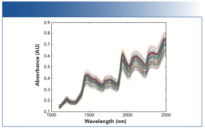
The need for data transformations did not develop in isolation. Nobody sat down one day and mused “Gee, I wonder if I could change these spectra I collected from my samples into other spectra, and what would happen if I did?” In isolation, such musing is pointless. Rather, the need or desire to change, or modify the spectra in a set, mainly grew out of the desire to improve analytical calibration performance and the need to be able to transfer calibration models between instruments and have them perform adequately well on the instrument to which the model was transferred. A particular need was for a calibration model to give the same answer when the same sample was measured a second time even when the sample was “repacked” (that is, removed from the sample holder and then replaced in it). The typical behavior of samples under those conditions is presented in Figure 1.

FIGURE 1: Overlayed spectra showing the variations because of repack or particle size effect. The samples in this case were ground wheat. As shown here, variations because of particle size effect can typically be larger than the spectral variations related to changes in the composition of the samples.

Thus, the question of data transformation is a subset of the questions revolving around the issues dealing with calibration transfer. We discussed the topic of calibration transfer previously and listed the various ways that goal can be (and has been) discussed by ourselves (2–8) as well as others. A good sampling of these methods can be found in the various “Theory and Application” articles referenced in the literature (9).

The ability to transfer calibrations between instruments certainly requires the hardware to be compatible, and we previously discussed that requirement as well (4,5). The reader also needs to consider the work done by Peter Griffiths (described in a later column of this subseries), wherein he explains how to convert spectra measured on an Fourier transform infrared (FT-IR)-based spectrometer to the equivalent spectra that would be obtained from a dispersive spectrometer, and vice versa.

However, the long history of calibration transfer when applied to near-IR (NIR) data indicated that having the hardware matching between two instruments is not always sufficient to ensure that a calibration developed on one instrument will perform comparably when used in conjunction with a different instrument, even one of the same make and model. One reason why that may occur is explained in our previous column (10). However, the figure in that previous column also illustrated a different point—when the data are highly correlated, the performance of almost any calibration model can be equivalent despite the wide differences of the actual calibration coefficients. It even becomes unclear as to whether the calibrations are “the same” or not. For this reason, data transforms are sometimes applied so that not only the calibration models perform similarly, but that they will do so when the models utilize the same (or nearly the same) calibration coefficients.

To avoid belaboring this issue, we concentrate on various data transformations that have been developed and applied, both by ourselves and other scientists. We avoid including the “derivative” transform (dⁿA/dλⁿ), the most common data transform used in NIR practice for several reasons. One reason is that this transform has been extensively discussed, both by others and by ourselves. We also avoid extensive discussion of the basic multiple linear regression (MLR) calibration algorithm for the same reason (11–20). Several chapters (4–7, 21, and 55–59) in the eponymous book based on this series of columns also discusses this derivative transform extensively (21).

Another reason is that, as the title of this column indicates, we are concentrating on data transforms that are used in conjunction with instruments that measure spectra at a limited number of discrete wavelengths (that is, interference filter-based instruments). Derivative transforms are not suited to such data because the use of a limited number of discrete wavelengths limits how closely together the wavelengths can be. Therefore, this occurrence forces the algorithm to violate the fundamental operation required by the definition of a “derivative”, that ΔX (in the denominator of ΔY/ΔX) is zero.

The whole concept of describing “derivatives” in connection with measured spectroscopic data is fraught with complications. Although never discussed in the chemometric literature or in the spectroscopic literature, the mathematical definition of a derivative is:

When applied to actual measured data that are typically digitized values from the measurement by an instrument, however, ΔX (or ΔY, for that matter) can never be zero, and the mathematical operation of taking the data to the limit of lim ΔX→0 can never actually be performed because in digitized data, there must always be a minimum difference of at least one digital bit between two successive numbers. However, the mathematics community has examined the issues that arise when data is digitized. One fundamental issue that needs to be dealt with is nomenclature: the term “derivative” should not be used in conjunction with digitized data. The mathematics community has replaced the term “derivative” (and “differential equations”) with the more accurate terms “differences” and corresponding “difference equations” (22) when digitized data is being considered. The spectroscopic and chemometric communities would do well to follow that lead.

Other Problematic Issues in Using “Derivatives”

One of the first things we learned about derivatives in calculus I after the basic concept and nomenclature was the property of the derivative that, if the data is multiplied by any constant, then the derivative of that data is multiplied by the same constant. In itself, this rule is not a problem because a computer will make the correct calculation for the data given, but when a “derivative” data transform is applied to a set of NIR calibration data, then the common claim that the “derivative” data transform “corrects for offset and scale differences between spectra” becomes inaccurate. “Scale” differences would automatically be included in the computation of the calibration coefficients.

A more serious problem arises when automated search algorithms are used to select the wavelength and the Δ (wavelength) representing the intended “derivative.” Because the underlying absorbance bands are usually nonlinear functions of the actual physical properties they are intended to represent, the application of linear mathematical algorithms introduced errors into the results obtained. These errors would typically be small, but we never really know in any particular case how severe this effect would be. For example, we would like to think that doubling the Δ (wavelength) would double the computed “derivative” (or at least the numerator term, especially in those software packages that do not perform the division by ΔX), but this outcome rarely occurs. We examined this situation in the past and presented the results (12–16), which showed that the accumulation of errors included the creation of artifacts (artificial spectral features that do not represent any actual physical phenomena).

Computing a calibration model based on “derivative” (actually difference) values produced a model that is effectively the same as a restricted version of MLR that is no longer a true least squares model that would be obtained from the original spectral data. Let us see how this comes about: Let S_i represent the various original spectral readings, and the corresponding model C = b₀ + b₁S₁ + b₂S₂ + b₃S₃ + b₄S₄. If, instead of computing a model based on the original data values, we convert the original spectral data to their differences (D₁ = S₂ − S₁, D₂ = S₄ − S₃), the resulting model for the differences becomes:

Because D₁ and D₂ are the differences of the original spectra data, this equation is actually equal to:

or, upon expanding the parenthesized terms:

Therefore, the calibration model expressed by equation 3 can be seen to have the same nominal form as a true least squares model, but it is not a true least squares model because the coefficients of S₁ and S₃ are restricted to being the negatives of the coefficients of S₂ and S₄. Therefore, they do not attain their true least squares values. Thus, we can expect that a model based on differences would be less accurate than a true least squares model; therefore, one would be better off to perform MLR on the original spectral data.

A common template followed by many modern applications papers is to collect data, perform calibration and validation calculations with and without the application of a hypothesized “repack correction” algorithm, compute the standard error of predictions (SEPs) corresponding to the two sets of calculations, and, if the SEP corresponding to the use of the repack correction algorithm is smaller than the SEP obtained without that “correction,” conclude that the “correction” is in fact performing its intended function. There are several problems with this scenario, any of which could negate the validity of the procedure.

SEP is indeed an important statistic for evaluating calibration performance, but it is being misused and misinterpreted when applied to the individual pieces of variance that contribute to the total error (such as the repack error). Because repack represents only a small fraction of the total error, true changes in the value of the error because the application of a “correction” procedure can be easily overwhelmed by changes in other (larger) error sources in the overall procedure, which can lead to false conclusions regarding the role of the correction procedure.

A better approach is to collect appropriate data and use the statistical procedure of analysis of variance (ANOVA) to directly calculate the contribution of repack variation (error) to the Total Error Sum of Squares of the calibration process, which can be done without and with the use of the correction procedure. The ANOVA would then directly provide values for the repack error that can legitimately be compared. However, this comparison is not a simple “is A > B?” comparison. Because this procedure involves the comparison of variances, a statistical F-test is necessary to properly compare the variances and determine if the procedure using the “repack correction” provides a statistically significant decrease in the repack error compared to the value obtained without the correction.

A still better approach is similar to the one above, but instead of calculating the contribution to the total error of the calibration, it is only necessary to determine the change in the readings when a sample is repacked. These changes can be averaged over the samples in the sample set (watch out for the signs of the changes for each sample!) again, with and without the correction procedure. This procedure is preferred because it can be performed using the statistical t-test rather than an F-test. Again, no conclusion can be drawn unless the reduction in the amount of repack variation is statistically significant.

We’ve decided to not discuss the most popular and common data transform and (arguably) one of the most common calibration algorithms. We will find out what that calibration algorithm is beginning in our next session, where we will start to examine alternate data transform methodologies including an algorithm that will make an MLR model based on data with special characteristics immune to the effect of repack.

Variations on the Algorithm

For starters, even though we did not discuss the MLR algorithm itself, there are a large number of algorithms based on variations of the MLR algorithm. These variations give the resulting calibration model special properties in addition to the least squared error property that the basic MLR algorithm provides. In the following discussions, A_i,j is the absorbance of ith ingredient at the jth wavelength, C is the concentration of the analyte, and b represents the calibration coefficient.

Variation #1 of the MLR Algorithm: b₀ = 0

Where and how and why does this arise? Statisticians have examined this case in detail, a good example discussion can be examined in chapter 19 of reference (23), dealing with mixture designs of experiments, particularly on pages 409–414. Mathematically, this forces the model to pass through the origin of the coordinate system. The authors point out that, because the sum of the ingredients in a mixture always equals 1 (unity), the dimensionality of the data from a mixture is always at least one fewer than the number of ingredients. Because of this rule, one cannot simply model the response variable (the constituent in an MLR model) using the compositions or, equivalently, an optical measurement representing those ingredient compositions, which is because of the fact that σ (ingredients) = 1 creates a perfect intercorrelation between the ingredients. Therefore, attempts to perform MLR on such data will inevitably result in a divide-by-zero error when performing the matrix inversion operation during the calibration.

One obvious way to break the intercorrelation between the ingredients is to leave one of the variables out of the calculations. This strategy will succeed (unless the data contains some other correlations between two or more of the remaining ingredients), but has some drawbacks:

• The calculations cease to be objective. Particularly at the beginning of a study, there are no objective ways available for guidance as to which ingredient (or ingredients) to omit, and then the choice of which ingredient to leave out of the calculations becomes subjective.
• The ingredient removed from the calculations may be a key predictor variable, so that removing its contributions to the data set will result in suboptimal results.
• To avoid the issue raised by the previous point (b), it will become necessary to perform trial calibrations, wherein each of the ingredients is successively removed from the data set, which would require increasing the amount of computation by a factor of at least m, where m is the number of ingredients in the mixture.

Draper and Smith (23) present an extensive discussion of this situation and propose that instead of removing any of the variables representing the ingredients from the calculations, the mathematics of the least square approach should be modified to remove the constant term from the model; that is, instead of the model being expressed as:

the model becomes:

This change was not completely original to Draper and Smith but represents the consensus of the statistical community at that time.

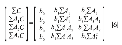
Note that equation 5 is not simply equation 4 with the b₀ term erased. It certainly looks like that, but the difference can be better appreciated by considering the normal equations from the two different approaches. The normal equations resulting from equation 4 (standard MLR) is:

In shorthand matrix notation, solving equation 6 for the values of the coefficients is expressed by the equation:

while the normal equations resulting from equation 5 (missing b₀) is

Interestingly, solving equation 8 for the coefficients results in the same matrix equation:

as for the previous conditions. The differences come from the construction of the equations (and matrices) themselves, to start with.

Equations 7 and 9 both come from performing the same operations on their respective models: they compute differences between the actual and predicted values from the model, sum the squares of the differences, then take derivatives with respect to each variable, and set the derivatives equal to zero. However, by eliminating the constant term, the matrix on the right-hand side of equation 8 loses an entire row and column compared to equation 6. Thus, even though what remains is the same as in equation 6, there is a whole group of computations that are not performed when the matrix is inverted, which affects all the subsequent results. Thus, the result of eliminating these computations cannot be replaced simply by eliminating b₀ from equation 1. The reason is that including the otherwise omitted computation results in different values for all the coefficients other than b₀, in addition to b₀ itself.

The formation and properties of least squares models without b₀ is discussed extensively in the statistics literature (23) as well as in the NIR literature (see Chapter 12 in (24)), a book on which some of this discussion is based). Here, we present it simply as another alternative way to calibrate NIR spectrometers. We think it is one of the many explorations performed by the early NIR practitioners and, although ignored, is worthy of further examination by the NIR community like in the case of several of the algorithms we examined here. In our next column on this topic, we will present and discuss another “simple” variation of MLR by adding the requirement that b_i = 0.

Validation of Linearity

Several years back, we wrote a series of columns examining classical least squares (CLS) analysis of liquid mixtures, culminating in a study where we demonstrated that volume fractions were the proper units in which to measure concentrations to use when calibrating spectroscopic instruments used for quantitative analysis of liquids (25). These results were also published in the formal literature (26) as well as Chapters 90–100 and 107–111 in the eponymous book (21). In these publications, we also conjectured that the use of volume fractions as the measure of “concentration” was also the solution to the “mystery” of the nonlinearity of Beer’s law. It has been well-known since the time that August Beer declared that absorbance was proportional to concentration that the relationship was true only for low concentrations of a solute (and correspondingly low values of absorbance), and that departures from that proportionality were observed when the concentration exceeded a defined threshold (which depended on the solute). Our conjecture, which was based on the additional fact that the various units that chemists used to express concentration (molarity, molality, weight fraction, mg/mL) are not all linearly related to each other, was that the same effect (use of an incorrect measure for “concentration”) was also the cause of the nonlinearity observed when various solutions were measured spectroscopically, and that use of volume fractions as the concentration measure should correct the nonlinearity observed in this situation as well. This conjecture was investigated by a group of European scientists (27), who confirmed that expressing “concentration” as volume fractions provided a graph with a linear relationship between concentration and absorbance, and other measures of concentration resulted in a nonlinear relationship. Additionally, Thomas Meyerhofer has studied and published extensively concerning the optical behavior of liquid mixtures, with a view to relating that behavior, and the linearity of the relationships to underlying fundamental physical properties (index of refraction, polarizability) of the ingredients as well as extensive previous work (28–30; in reference [30], Meyerhofer demonstrates that Beer's Law follows from the fundamental physics when concentrations are expressed as volume fractions).

References

(1) Eastern Analytical Symposium, NY/ NJ Section of the Society for Applied Spectroscopy Gold Medal Award (accessed May 2022). https://eas.org/2020/?p=5502

(2) H. Mark and J. Workman Jr., Spectroscopy 28(2), 24–37 (2013).

(3) J. Workman Jr. and H. Mark, Spectroscopy 32(10), 18–25 (2017).

(4) J. Workman Jr. and H. Mark, Spectroscopy 33(6), 22–26 (2018).

(5) J. Workman Jr. and H. Mark, Spectroscopy 28(5), 12–21 (2013).

(6) J. Workman Jr. and H. Mark, Spectroscopy 28(6), 28–35 (2013).

(7) J. Workman Jr. and H. Mark, Spectroscopy 28(10), 24–33 (2013).

(8) J. Workman Jr. and H. Mark, Spectroscopy 29(5), 18–27 (2014).

(9) E.W. Ciurczak, B. Igne, J. Workman Jr., and D.A. Burns, eds., Handbook of Near-Infrared Analysis, Fourth Edition in Practical Spectroscopy Series (CRC Press imprint of Taylor & Francis Group, Boca Raton, FL, 2021), pp. 808.

(10) H. Mark and J. Workman Jr., Spectroscopy 37(2), 16–18,54 (2022).

(11) J. Workman Jr. and H. Mark, Spectroscopy 12(5), 32–36 (1997).

(12) H. Mark and J. Workman Jr., Spectroscopy 18(4), 32–37 (2003).

(13) H. Mark and J. Workman Jr., Spectroscopy 18(9), 25–28 (2003).

(14) H. Mark and J. Workman Jr., Spectroscopy 18(12), 106–111 (2003).

(15) H. Mark and J. Workman Jr., Spectroscopy 19(1), 44–51 (2004).

(16) H. Mark and J. Workman Jr., Spectroscopy 19(11), 110–112 (2004).

(17) D. Hopkins, NIR News 12(3), 3–5 (2001).

(18) D. Hopkins, J. Korean Soc. Near Infrared Anal. 2(1), 1–13 (2001).

(19) D. Hopkins, Near Infrared Anal. 2(1), 1–13 (2001).

(20) D. Hopkins, NIR News 27(7), 23–28 (2016).

(21) H. Mark and J. Workman Jr., Chemometrics in Spectroscopy (Elsevier, Amsterdam, The Netherlands, 2nd ed., 2018).

(22) B.W. Arden, An Introduction to Digital Computing (Addison-Wesley Publishing Co., Inc., Reading, MA, 1st ed., 1963).

(23) N. Draper and H. Smith, Applied Regression Analysis (John Wiley & Sons, New York, NY, 3rd ed., 1998).

(24) H. Mark, In Handbook of Near-Infrared Analysis (CRC Press; Boca Raton, FL, 4th ed., 2021).

(25) H. Mark, Spectroscopy 29(5), 18–40 (2014).

(26) H. Mark, R. Rubinovitz, D. Heaps, P. Gemperline, D. Dahm, and K. Dahm, Appl. Spectrosc. 64(9), 995–1006 (2010).

(27) H.Y.M. Yan, Z. Xiong, H. Siesler, L. Qi, and G. Zhang, Molecules 24(19), 3564 (2019).

(28) T. Meyerhofer and J. Popp, Appl. Spectrosc. 74(10), 1287–1294 (2020).

(29) T. Meyerhofer, S. Pahlow, and J. Popp, Chem. Phys. Chem. 21(18), 2029–2046 (2020).

(30) T. Meyerhofer, I. Oleksii, A. Kutsyk, and J. Popp, Appl. Spectrosc. 76(1), 92–104 (2022).

Howard Mark serves on the Editorial Advisory Board of Spectroscopy, and runs a consulting service, Mark Electronics, in Suffern, New York. Direct correspondence to: SpectroscopyEdit@mmhgroup.com

Jerome Workman, Jr. serves on the Editorial Advisory Board of Spectroscopy and is the Senior Technical Editor for LCGC and Spectroscopy. He is also a Certified Core Adjunct Professor at U.S. National University in La Jolla, California. He was formerly the Executive Vice President of Research and Engineering for Unity Scientific and Process Sensors Corporation. ●