Evaluating a Multilayer Polymer Film by Raman Microscopy
Multilayer polymer films are engineered to accommodate a variety of requirements where polymer layers are fused together, with each polymer selected for a specific purpose. Specific analysis approaches can troubleshoot a defective film or allow us to reverse-engineer a film of unknown composition. Since the inception of Raman microscopy in the mid-1970s, it has been argued that a well designed confocal Raman microscope can analyze the composition of a multilayer film non-destructively. This is a powerful capability because it has the potential to provide information with optical resolution (better than 1 μm) below sample surfaces non-destructively. However, because standard microscope optics do not maintain focus inside of a material with a finite index of refraction, and the errors become greater with increasing numerical aperture and increasing depth, we wanted to determine the quality of the information achieved by comparing a depth profile with a two dimensional map of a cross-section. In this article, we show a cross-sectional map of a film compared to a depth profile to evaluate the quality of depth profile measurements.
In 2000, Neil Everall at the United Kingdom’s Imperial Chemical Industries showed that a dry objective, which is standard in Raman microscopes, cannot maintain focus inside a material with a non-unitary index of refraction (1). Recognizing that there are objectives available that can better match a sample’s optical characteristics, we tested and demonstrated that an objective with a cover-glass correction vastly improved the signals from a gaseous inclusion in a glass sample (2).
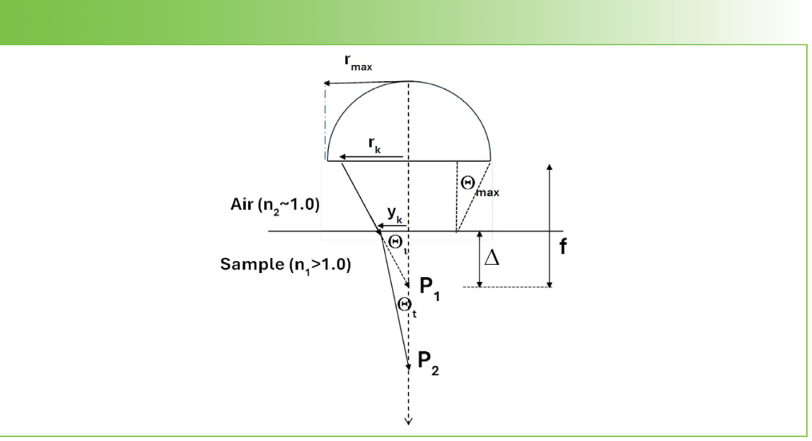
Figure 1 reproduces the principles from the Figure 1 in Everall’s publication and shows the origin of the problem clearly. As the light emerges from the last lens in the objective (represented by the semicircle in the figure), the light is focused at the point labeled P1 in the figure, if the focus is in air. As shown in the left part of the figure, when entering the sample, the light rays will be bent towards the normal at the interface, because of the refractive index mismatch, and the larger the angle hitting the interface, the larger the deviation. Because the objective defines a bundle of rays whose angle varies from 0 at the center to a maximum of Өmax, determined by the numerical aperture (NA) of the objective, the rays will not all merge at the same point P2. In fact, the larger the angle of the ray entering the sample, the deeper will be the focal point, P2. The irony is that one usually selects an objective for high NA to optimize spatial resolution, but, when focusing inside a material with a refractive index greater than 1.0, that focus will be degraded, and the degree of degradation will increase with the NA. The solution to this problem is to use an objective corrected for a finite index. Objectives corrected for use in water (whose refractive index is 1.33) or oil (refractive index about 1.5) are available. Because many polymers have refractive indices of approximately 1.5, an oil immersion objective is the better choice. The depth profile that is shown in this article was measured with an oil immersion objective.

.")
FIGURE 1: Ray trace of photon trajectories from a microscope objective into a material with an index of refraction > 1.0 (1).
Description of Sample
The sample measured was a commercial multilayer film that was held in a chuck designed specifically for handling such samples. After the film is mounted in the chuck, a fresh razor blade is used to make a clean cut parallel to the top surface of the chuck. The device is shown in Figure 2. Figure 3 then shows the optical image of the sample surface in the chuck.


FIGURE 2: Chuck for clamping laminated films and cross-sectioning. Note that the entire device can be rotated 90o so that the orientation behavior can also be investigated.
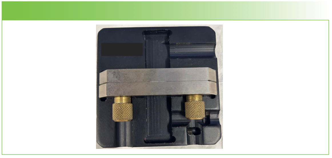

FIGURE 3: Sample cross-section measured with the 100x objective using the montage capability to splice adjacent regions accurately in order to create a final high-quality image.
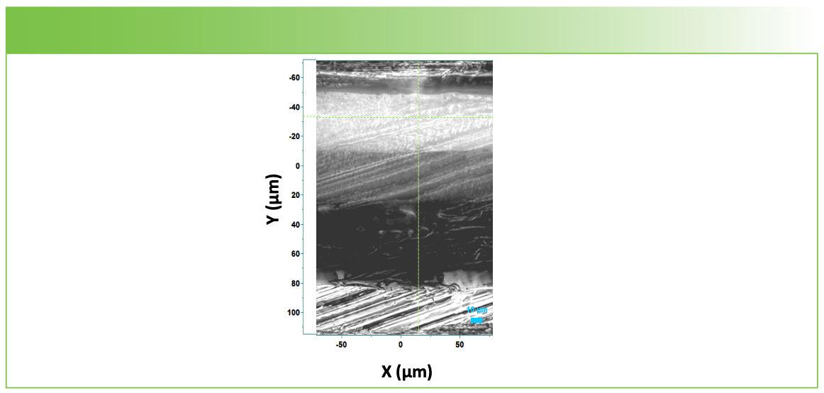
The microscope image shown in Figure 3 indicates the presence of at least four layers, but because of the low contrast and the possibility for the presence of thin layers, it will take Raman measurements to determine what is present. After we show the Raman map of the cross section, we show the results of the depth profile, and then, finally, plot the two profiles side by side for comparison. We consider the map of the cross section to be the gold standard indicator of the “truth,” against which the depth profile will be compared.
Cross-Sectional Map
The spectra were acquired with the 638 nm laser on the XploRA using the 600 g/mm grating which provided full spectra without scanning. The laser was used at 50% power, and autofocus capabilities were used at each spot. The step size between data points in the x direction was 2 µm, and in the y direction was 1 µm. The spectra were baseline-corrected, and then we applied multivariate algorithms. Sometimes, I surfed the spectra until I found what appeared to be “pure” spectra, and captured them for mapping using classical least squares (CLS). On occasion, I found that I was not able to separate the components to my satisfaction so I ran multivariate curve resolution (MCR), and was pleasantly surprised to find that it provided more acceptable results.
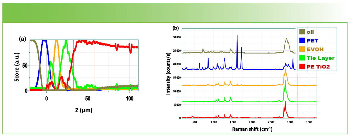
Figure 4a shows the spectra that the analysis revealed as “pure components.” The top spectrum is that of polyethylene. The next one down is also polyethylene, but with a significant contribution from TiO2, which is often added as a white pigment. The third spectrum down is polyethylene terephthalate. We believe that the next one is a tie layer, because it appears as a rather thin layer in the map. The fifth we believe to be polyvinyl alcohol. The two spectra at the bottom are that of a carbon and a very weak organic material. These two spectra actually appear on the metal, and we added them so that the software would not force fit spectra from the metal with the spectra of the polymers. Figure 4b shows the map next to the film cross section on which we drew a rectangle to represent the area where the mapping spectra were acquired.

 MCR factors that were automatically calculated by the software and used to construct the map in Figure 4b. (b) Microscope image of the sample cross-section (left) compared to the Raman map constructed using MCR factors from Figure 4a (right).")
FIGURE 4: (a) MCR factors that were automatically calculated by the software and used to construct the map in Figure 4b. (b) Microscope image of the sample cross-section (left) compared to the Raman map constructed using MCR factors from Figure 4a (right).
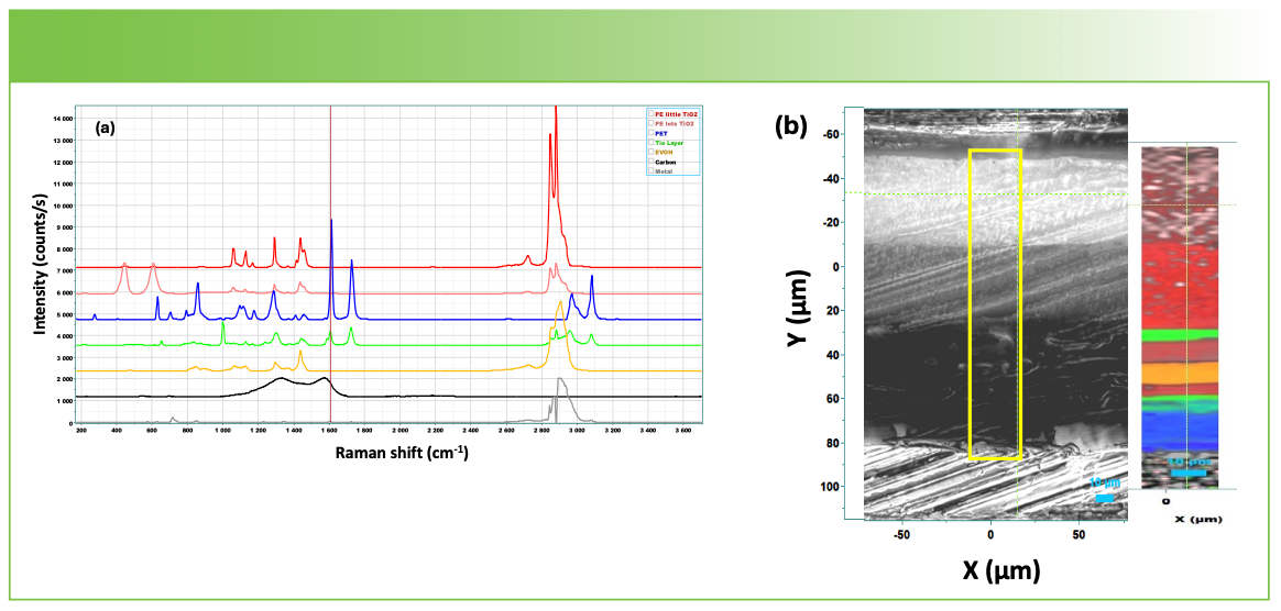
From top to bottom, the Raman map shows a layer of polyethylene, which contained a significant amount of TiO2, then polyethylene with much less TiO2, then what looks to be a tie layer, then a small layer of polyethylene, then a layer of polyvinyl alcohol, another thin layer of polyethylene, a tie layer, and then polyethylene terephthalate. Note that the polyethylene layer on the top of the map is dominated by the TiO2, and the spectrum of the polymer is much weaker than it is in the second layer down. This is clear by comparing the top two spectra in Figure 4a. Interestingly, this observation is consistent with the optical micrograph which shows the top layer with the TiO2 much whiter indicating light scattering.
Depth Profile
At this point, I will show the results of a depth profile of this same material in Figure 5. As I pointed out earlier, I found that the results were much improved when I used an oil immersion objective. These spectra were acquired with the same laser wavelength and grating, also with 50% laser power. The slit and hole were set to 50 and 100 µm, respectively (as they were for the cross section measurements), to optimize spatial resolution in the map. Note that, because the profile was started above the top surface of the film, the spectrum of the oil was also collected and is shown here.

 Depth profile of the polymer laminate constructed from the factors shown in Figure 5b. (b) Factors used to construct the depth profile shown in Figure 5a.")
FIGURE 5: (a) Depth profile of the polymer laminate constructed from the factors shown in Figure 5b. (b) Factors used to construct the depth profile shown in Figure 5a.
Comparison of the Results of the Cross-Sectional Map and the Depth Profile
Figure 6 shows the two results side by side with the dimensions of the displays adjusted so that they could be accurately compared. Note that I took some trouble to color-code the analogous layers with the same colors.


FIGURE 6: Comparison of the cross-sectional map acquired with the 100x objective to the depth profile acquired with the 63x oil immersion objective.
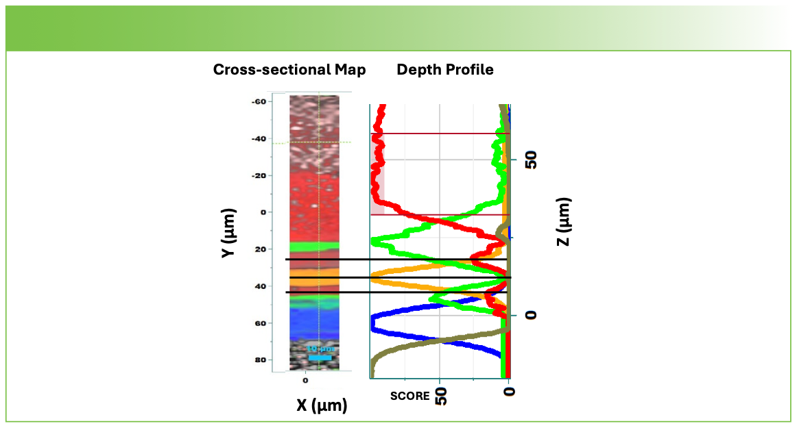
Let’s look at the differences. The first thing that you see is that the red polyethylene layer in the map seems to be thinner than the polyethylene in the depth profile. In fact, as we stated above, there are two polyethylene layers seen in the cross section, and the second one is dominated by the TiO2; this layer does not appear in the depth profile. Note that when we acquired the depth profile, we mounted the sample with the polyethylene terephthalate on top, so when the light was focused in the second polyethylene layer, there was so much light scattering that it probably could not penetrate. The signal just continued to drop, which we see if we plot non-normalized scores (not shown). However, the alignment of the layers is remarkably good. But when we look at the factors (the spectra), we do see some surprising differences.
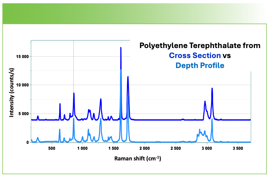
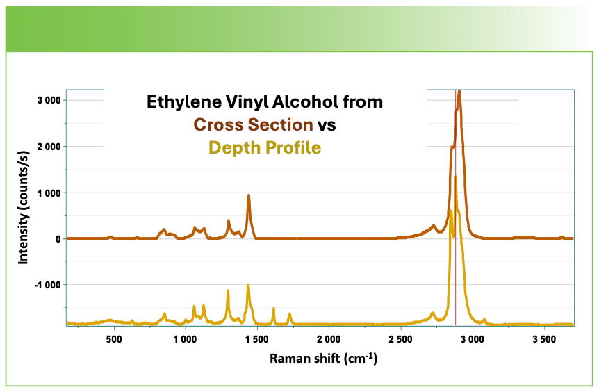
Note that even though the spectrum of polyethylene terephthalate in Figure 7 extracted from the depth profile was taken far from the polyethylene, there is a significant contribution from the polyethylene in that spectrum. I remember at a conference hearing Neil Everall saying that he was aware that even the best confocal measurements show evidence for material far from the plane from which the spectrum was generated. A similar comparison of the ethylene vinyl alcohol layer in the two measurements in Figure 8 show not only contributions from polyethylene terephthalate, but also from the polyethylene in the depth profile factor in the depth profile factor.

, and from the depth profile (bottom).")
FIGURE 7: Spectrum of polyethylene terephthalate layer extracted from the cross-sectional measurement (top), and from the depth profile (bottom).

, and from the depth profile (bottom).")
FIGURE 8: Spectrum of the ethylene vinyl alcohol layer extracted from the cross-sectional measurement (top), and from the depth profile (bottom).
Conclusions
The information provided by a depth profile Raman microscope measurement is not available by any other technique. This comparison shows that, when using an oil immersion objective, the behavior of the depth profile is quite similar to that of the cross section. However, the separation of the components is not quite as good in the depth profile as in the cross-sectional measurements. It is possible that, if one is careful selecting an immersion oil that matches better the polymers, there will be less mixing. Because there are instances where information of a laminated film is needed, but removing the film and cross sectioning it is not practical, a confocal depth profile is the preferred method for measurement. This comparison shows that this can be a practical approach, and what the limitations might be.
References
(1) Everall, N. J. Modeling and Measuring the Effect of Refraction on the Depth Resolution of Confocal Raman Microscopy, Appl. Spectrosc. 2000, 54 (6), 773–782. DOI: 10.1366/0003702001950382
(2) Adar, F.; Naudin, C.; Whitley, A.; Bodnar, R. Use of a Microscope Objective Corrected for a Cover Glass t Improve Confocal Spatial Resolution inside a Sample with a Finite Index of Refraction. Appl. Spectros. 2004, 58 (9), 1136–1137. DOI: 10.1366/0003702041959361


Fran Adar is the Principal Raman Applications Scientist for Horiba Scientific in Edison, New Jersey. Direct correspondence to: SpectroscopyEdit@mmhgroup.com. ●


AI-Powered SERS Spectroscopy Breakthrough Boosts Safety of Medicinal Food Products
April 16th 2025A new deep learning-enhanced spectroscopic platform—SERSome—developed by researchers in China and Finland, identifies medicinal and edible homologs (MEHs) with 98% accuracy. This innovation could revolutionize safety and quality control in the growing MEH market.


New Raman Spectroscopy Method Enhances Real-Time Monitoring Across Fermentation Processes
April 15th 2025Researchers at Delft University of Technology have developed a novel method using single compound spectra to enhance the transferability and accuracy of Raman spectroscopy models for real-time fermentation monitoring.

Nanometer-Scale Studies Using Tip Enhanced Raman Spectroscopy
February 8th 2013Volker Deckert, the winner of the 2013 Charles Mann Award, is advancing the use of tip enhanced Raman spectroscopy (TERS) to push the lateral resolution of vibrational spectroscopy well below the Abbe limit, to achieve single-molecule sensitivity. Because the tip can be moved with sub-nanometer precision, structural information with unmatched spatial resolution can be achieved without the need of specific labels.


