LIBS Basics, Part III: Deriving the Analytical Answer — Calibrated Solutions with LIBS

This installment is the third in a three-part series focusing on major aspects of laser-induced breakdown spectroscopy (LIBS). The first installment set the stage with the basics of the LIBS measurement physics and standard applications. The second installment discussed the choices and trade-offs for LIBS hardware in detail, in particular focusing on lasers and spectrometers. This third installment discusses LIBS analysis in some depth, exploring the various ways to go from a LIBS spectrum to a solution.

One of the strengths of laser-induced breakdown spectroscopy (LIBS) is that it can be applied to multiple media. In various configurations, it is possible to measure solids, liquids, gases, and suspended aerosols. Measurements have been made on the ocean floor at depths of hundreds of meters, and on the surface of Mars in an atmosphere of 7 Torr, largely consisting of CO₂. This flexibility is possible because the atomization and excitation source are combined in the LIBS laser pulse. This strength of LIBS is a complication, however, because the material ablation and plasma formation process profoundly impacts the analytical plasma, as we pointed out in the previous installments in this series (1,2). As a result, users must be careful when developing material classification and calibration methods for LIBS, in particular using "like" materials for calibrations and choosing methods consistent with the type and range of expected data. While it is impossible to cover the gamut of considerations in a short column installment, here I will attempt to cover some major features of the calibration and classification landscape.

Basic Calibration

Any discussion of calibration should start with univariate analysis of spectral peaks, the primary method of calibration of spectroscopic output since such analysis has been attempted. Spectral peak analysis in the context of LIBS spectra has a number of considerations. First, astute readers will note that the LIBS plasma is a time-dependent event. The acquisition period of the spectra relative to the plasma initiation becomes an important parameter in the quantification. This collection period is also a function of the laser energy density on the plasma, because the plasma lifetime scales with the deposited energy in the plasma, and the ablation event is important (primarily for solids) not only for exciting analytes, but also in determining the amount of laser energy channeled into the plasma. Hence, any calibrated LIBS system should take care to ensure consistent laser fluence (energy/area) on the samples.

The influence of the data collection timing has been shown often, for example in an early paper by Fisher from Hahn's group (3). Figure 1 shows the chromium emission lines from particles in an airborne aerosol at three different settings of delay (after the plasma initiation) and gate width (shutter open time), collected with a Czerny-Turner spectrometer and an intensified charge-coupled device (ICCD) camera. At 2 μs delay and gate, the chromium triplet is not visible at all. At later times and longer collection periods, the signal-to-noise ratio (S/N) of the triplet is optimized. Fisher's paper goes on to point out that the optimum detector timing to maximize S/N is element-dependent under otherwise constant experimental conditions.

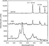
Figure 1: Spectra of chromium aerosol collected at different delay/gate combinations, indicated by delay/gate in microseconds to the left of each spectrum. Spectra are offset for clarity, but are otherwise the same scale. Adapted from reference 3 with permission.

After the data collection (laser energy, spot size, and collection timing) is fixed, data can be collected from known samples to form a calibration curve. Typically, a particular peak is selected for analysis of an element of interest. As shown in Figure 2, the peak (blue, solid fill) is defined and integrated, with the subtraction of the background, which can be defined by the area under the peak, defined by the peak edges (green, grid fill), or by nearby areas with no spectral interferences (orange, diagonal fill). Sometimes the peak area alone can be used for calibration, but in other cases the peak is divided by the background, sometimes called the "baseline," to form the "peak/base" ratio. If the spectrum is collected at proximate enough time to the plasma that there is a measurable continuum, this peak/base calibration tends to work well, because the baseline is indicative of the energy absorbed in the plasma. In other cases, normalization of the peak by the total plasma emission (Figure 3a) can be useful if the total plasma emission is fairly constant (for example, measurement of a low concentration alloying element in a steel matrix). If there is a known, fairly constant element, another similar approach is to use a line of the constant element to standardize the peak of the element of interest (Figure 3b). For groups of samples with a consistent or relatively simple background, univariate methods are often very successful calibration schemes for LIBS.

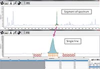
Figure 2: Example of peak integration and baseline (background) definitions.

Extensions to Basic Calibration — Line Selection

Individual emission lines each have a particular range of applicability. Lines with low excitation energy and ending at or near the ground state tend to have a nonlinear response at higher concentrations because of self-absorption, but these lines are the most sensitive for measurements at low concentrations. Harder-to-excite lines, particularly those not ending on the ground state, are more useful for higher-concentration measurements. Lines not ending on the ground state are not as susceptible to self-absorption as lines that transition to the ground state (there is negligible population to absorb in upper states). The result of these factors is that calibration lines are selected based on the concentration range being measured, and often the strongest lines in the spectrum of a particular element are not used for higher-concentration measurements. Similar to inductively coupled plasma (ICP) methods, calibration over a large range of analyte concentrations may use a succession of lines, some for lower concentrations and some for higher concentrations.

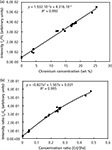
Figure 3: Univariate calibration of the (a) chromium 397.67-nm line divided by the total light intensity from the plasma, and the (b) chromium 397.67-nm line divided by the iron 404.58-nm line, in a range of low- to high-alloy steels. Adapted from reference 4 with permission.

Multivariate Calibration

Multivariate concentration methods use multiple lines, or multiple parameters, to come to a concentration measurement. Broadly, these methods are lumped under the heading of "chemometrics." The most common include partial least squares (PLS), principal component regression (PCR), and support vector machines regression (SVR). Numerous other methods exist, and additional methods are continuously under development. Those mentioned here are the ones most likely to be found in commercial data analysis packages and implemented in mathematical programming languages such as R, Python, or Matlab. The description of the methods below is merely to guide use and implementation, and the reader is encouraged to find additional resources for the study of particular methods of interest.

One commonality to all of these multivariate methods is the importance of the definition of a "training" set of data and a "test" set of data. This is more important for multivariate methods than for univariate peak integration because the predictive model is of arbitrary dimension using many of the multivariate techniques, and the number of sample spectra is relatively few compared with the number of data points in each spectrum. For example, an analyst may have 100 spectra for each of 10 different standards for calibration of a particular element in an alloy — seemingly a lot of data. However, each spectrum may itself have 10,000 or more data points, with each data point acting as an individual parameter, allowing arbitrarily complex modeling. Typically, as the number of predictive variables increases in the model, the better the performance is on the training data. The result is that complex models can be (and are, by hapless analysts) built using too many coincidently correlated variables. Such "over-fit" models may perfectly describe the training data, but will quickly fail on independent test data and on data that is slightly outside of the range of the training data. The remedy is rigorous testing with independent test data to ensure that the model is stable and accurate when presented with new challenges. During the model-building phase, one can and should use a cross-validation method (such as leave one out, k-fold cross-validation, and so on). One is reminded otherwise of the quotation attributed to John von Neumann: "With four parameters I can fit an elephant, and with five I can make him wiggle his trunk" (5).

As suggested above, it is usually a good strategy to limit the number of predictive variables to the minimum number required to sufficiently model the data, thus ensuring that the model takes only "primary" features into account. One other means of accomplishing this is to preselect important lines or portions of the spectrum, potentially also pretreating the data, before sending the data to a multivariate technique for calibration. In this way, the physical aspects of the data can be emphasized (for example, several Mg emission peaks can be used to predict Mg), which tends to increase the accuracy of the model compared to models that use a general method to determine which variables are most correlated. An example of this is data treated using the PLS "dominant factor" method promoted by Wang and colleagues (6), in which preselected factors (for example, normalized peaks or plasma parameters) are emphasized in the PLS. Figure 4 shows PLS-based calibrations derived from 77 standard coals, in which the LIBS predicted value is on one axis, and the known value is on the opposite axis. Figure 4a is a prediction of carbon in coal using only PLS on the more than 13,000 values in the original spectra. Figure 4b shows preliminary data showing dominant factors PLS data, using primarily the roughly 200 most important lines in the spectra, standardized. Obviously, a significant improvement can be achieved with "smart" inputs to a multivariate method like PLS.

Figure 4: Predictions of carbon concentration compared with actual values in 77 coal samples using (a) standard PLS on the raw coal data (by the author), and (b) dominant factors PLS (preliminary data from the laboratory of Professor Zhe Wang, Tsinghua University). In (a) "x" marks training data and dots indicate test data, while in (b) "+" marks the training data and squares indicate test data.

In terms of the methods, given x and trying to predict y, PLS attempts to find those factors, called latent variables, that best describe the variation in the training set. The first latent variable describes the maximum amount of variation in y, and subsequent latent variables are orthogonal to previous latent variables, each describing the maximum amount of remaining variation in x. Users should note that PLS is inherently a linear multivariate method, and so substantial nonlinearity in the relationship between x and y will be difficult to capture. However, PLS is excellent for datasets in which there are multiple related variables (as in many pixels related in a particular atomic peak), and in which there are many more variables than observations. As both of these conditions are true of LIBS, PLS is commonly used for LIBS calibrations. PCR is a related method.

Support vector machines (SVM) can be used for classification or for regression, termed support vector regression (SVR). Data are projected into higher-dimensional spaces to achieve separation, and discrimination is made by determining the separation between data in those higher-dimensional spaces. Kernels for data projection can be either linear or nonlinear, enabling SVM-based methods to deal with both types of data, provided that the appropriate kernel is chosen. Figure 5 illustrates SVR used on the same coal dataset mentioned above, in which the line represents the model built with the training data, and the points represent the prediction on the test set. This prediction used a linear kernel on the raw LIBS data.

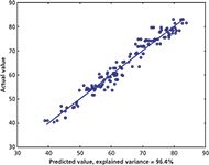
Figure 5: SVM regression of the raw coal data from the dataset described earlier, by the author. The blue line is the model from the training data and the points are from the test set of data.

Classification

Classification is often a simpler problem than quantification. These problems involve simple identification of a sample and placing it into one of a set of known classes. Multivariate classification methods are likely more numerous than multivariate quantification methods, and again readers are encouraged to find additional resources for self-study. Popular classification methods include clustering, soft independent modeling of class analogy (SIMCA), partial least squares discriminant analysis (PLS-DA), and the previously mentioned SVM.

Of all of the methods, clustering methods are one of the simplest. In a typical clustering method, the centroid of a group of M spectra of N points would be calculated by determining the average value of each of the N pixels. The M spectra would all be of the same type. With the centroid of every type (class) of sample calculated, the model can be run on unknowns. For each unknown, a "distance" such as the Euclidean distance (root-square calculated with each of the N pixels of the unknown spectrum) from the unknown to each of the class centroids is calculated. The class with the centroid that is closest to the unknown is deemed the class of the unknown. In this way, every unknown is assigned to a class. Variants include alternative methods of distance calculation, and definition of threshold distances that define when an unknown is a member of a class (and outside of which the unknown may be assigned to an "unknown" class).

SIMCA relies on a principal components analysis (PCA) to separate known materials into classes. Because SIMCA is a supervised method that is given the class of each of the known training samples when building the model, it retains only those principal components that are useful in predicting class. When presented with unknowns, it can predict the probability that the unknown is a member of one of the classes, or it can predict that the unknown is not in any of the known classes, depending on the tolerances that are set during building of the model.

PLS-DA uses the same methods as PLS to project the data into latent structures. Instead of continuous variables for quantitative prediction, discrete variables are assigned for classification.

Most classification results are either presented in terms of a "confusion matrix" or a receiver operating characteristic (ROC) curve, which graphs the false positive rate (x-axis) versus the true positive rate (y-axis). An example of a confusion matrix is shown in Figure 6. In this figure, samples are given arbitrary class names 1, 3, 5, . . . 17, and 21. The actual data that generated this matrix were types of fertilizer and the test set were five samples of each type. A K-nearest neighbor (KNN) clustering algorithm was used to try to place unknowns into classes. Numbers on the diagonal of the matrix indicate correctly identified samples — that is, three samples that were actually in class "1" were also identified as class "1," and five samples that were actually in class "13" were identified as class "13." Misidentifications are off of the diagonal, such as the two samples of class "1" that were predicted to be class "3," or the one sample (each) of class "5" that were predicted to be class "3" and class "7." In this case, the samples were ordered by increasing nitrogen concentration and decreasing phosphorous concentration, so all of the confusions were from the correct class to the adjacent class. On the same data, a perfect classification (all "5's" on the diagonal) could be achieved with the SIMCA algorithm.

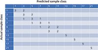
Figure 6: A confusion matrix representing performance of a clustering algorithm on LIBS analysis of fertilizer samples.

Hybrid Schemes

Methods can be combined to improve accuracy. As an example, a classification might be used to separate samples into logical groups before applying more specific quantitative calibrations developed for each group. Or a statistical method such as analysis of variance (ANOVA) could be used to determine the independent variables (intensities) in a spectrum that are most closely correlated to a dependent variable that one is trying to predict, and those variables could be fed into a quantitative method such as PLS. The possibilities for variation are endless, as are the pretreatment methods for spectra, such as normalization, averaging, and so forth. I encourage readers to explore and try different methods, particularly realizing that each dataset may require slightly different treatment.

"Calibration Free" LIBS

A discussion of LIBS calibration methods would not be complete without a mention of so-called "calibration-free" LIBS. These methods generally aim to derive fundamental parameters from the plasma, such as equilibrium temperature and electron density. They use these parameters in conjunction with the emission spectra to "close the loop" on overall element concentrations, assuming that all major elements in the sample can be measured.

For example, if the plasma conditions are known, then for a single element the ratios of atomic lines in the spectrum can be predicted. For two elements in a binary system, the relative emission coefficients between various major lines of each of the elements are known, and so the relative concentration (which would add up to 100%) in the binary system is known. For 3, 4, . . . N elements, there are more equations but the method is the same, the closure condition being that the predicted concentration of the N elements should add up to 100%.

Great strides have been made in calibration-free methods, notably by researchers from Pisa (7) and with useful additions by Gornushkin and coworkers (8). Accuracies in known systems can be ±20% or better. Issues with the method include uncertainties in the relative emission coefficients, inter-element interactions, and uncertainties in the plasma parameters. Plasma conditions are not stationary during any detection interval of finite duration, nor are plasma temperature and electron density homogenous in the plasma volume. Adjustments for these time- and space-dependent distributions have been helpful in advancing the method, which remains an active area of research.

Summary

There are obviously many methods to come to both quantitative calibration and qualitative classification with LIBS. I am often asked what to expect in terms of overall performance. With real-world samples, typical relative standard deviation (RSD) numbers are in the range of 2–3% for many types of analysis. For the most homogenous samples, RSDs less than 1% can be achieved, for example, on obsidian glass samples or gemstones. With both classification and quantification methods, one must be sure to avoid over-fitting and rigorously test any model before deployment. Following the general guidelines here, with a bit of experimentation, should get you a good way toward successful implementation of LIBS.

As this is the last of the three tutorial installments planned in Spectroscopy on LIBS, I'd like to express my appreciation to the editors for suggesting this series. It has been a joy to write. For those readers who have additional questions, please feel free to use my e-mail address listed on the next page. Those who know me will attest that I always enjoy talking about LIBS! Best of luck to each of you in your spectroscopic endeavors!

References

(1) S. Buckley, Spectroscopy 29(1), 22–29 (2014).

(2) S. Buckley, Spectroscopy 29(4), 26–31 (2014).

(3) B.T. Fisher, H.A. Johnsen, S.G. Buckley, and D.W. Hahn, Appl. Spectr. 55(10), 1312–1319 (2001).

(4) C.B. Stipe, B.D. Hensley, J.L. Boersema, and S.G. Buckley, Appl. Spectr. 64(2), 154–160 (2010).

(5) Attributed by E. Fermi, as quoted by F. Dyson in Nature 427, 297 (22 January 2004).

(6) Z. Wang, J. Feng, L. Li, W. Ni, and Z. Li, J. Anal. At. Spectrom. 26, 2289–2299 (2011).

(7) E. Tongnoni, G. Cristoforetti, S. Legnaioli, and V. Palleschi, Spectrochim. Acta B. 65(1), 1–14 (2010).

(8) I.B. Gornushkin, S.V. Shabanov, S. Merk, E. Tongnoni, and U. Panne, J. Anal. At. Spectrom. 25(10), 1643–1653 (2010).

Steve Buckley is a Director of Market Development at TSI Incorporated, which acquired the LIBS business of Photon Machines, Inc., in 2012. Before cofounding Photon Machines, Steve was a tenured professor of engineering at the University of California at San Diego. He has been working on research and practical issues surrounding the implementation of LIBS since 1998. He can be reached at steve.buckley@tsi.com

Steve Buckley