Limitations in Analytical Accuracy, Part II: Theories to Describe the Limits in Analytical Accuracy and Comparing Test Results for Analytical Uncertainty

Limits in Analytical Accuracy

You might recall from our previous column (1) how Horwitz throws down the gauntlet to analytical scientists, stating that a general equation can be formulated for the representation of analytical precision based upon analyte concentration (2). He states this as follows:

CV(%) = 2^{(1–0.5logC)}

where C is the mass fraction as concentration expressed in powers of 10 (for example, 0.1% analyte is equal to C = 10^–3).

A paper published by Hall and Selinger (3) points out an empirical formula relating the concentration (c) to the coefficient of variation (CV), also known as the precision (σ). They derive the origin of the "trumpet curve" using a binomial distribution explanation. Their final derived relationship becomes

They further simplify the Horwitz trumpet relationship in two forms as follows:

CV(%) = 0.006c^–0.5

and

σ = 0.006c^0.5

They then derive their own binomial model relationships using Horwitz's data with variable apparent sample size.

CV(%) = 0.02c^–0.15

and

σ = 0.02c^0.85

Both sets of relationships depict relative error as inversely proportional to analyte concentration.

In yet a more detailed incursion into this subject, Rocke and Lorenzato (4) describe two disparate conditions in analytical error: concentrations near zero and macro level concentrations, say greater than 0.5% for argument's sake. They propose that analytical error comprises two types, additive and multiplicative. So their derived model for this condition is

x = μe^η + ε

where x is the measured concentration; μ is the true analyte concentration; and η is a normally distributed analytical error with mean 0 and standard deviation σ_η. It should be noted that η represents the multiplicative or proportional error with concentration and ´ represents the additive error demonstrated at small concentrations.

Using this approach, the critical level at which the CV is a specific value can be found by solving for x using the following relationship:

(CVx)² = (σ_ηx)² + (σ_ε)²

where x is the measured analyte concentration as the practical quantitation level (PQL used by the U.S. Environmental Protection Agency [EPA]). This relationship is simplified to

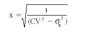
where CV is the critical level at which the coefficient of variation is a preselected value to be achieved using a specific analytical method, and σ_η is the standard deviation of the multiplicative or measurement error of the method. For example, if the desired CV is 0.3 and σ_η is 0.1, then the PQL or x is computed as 3.54. This is the lowest analyte concentration that can be determined given the parameters used.

The authors describe the earlier model as a linear exponential calibration curve as

y = α + βμe^η + ε

where y is the observed measurement data. This model approximates a consistent or constant standard deviation model at low concentrations and approximates a constant CV model for high concentrations. In this model, the multiplicative error varies as μe^η.

Detection Limit for Concentrations Near Zero

Finally, detection limit (D) is estimated using

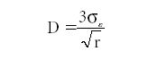
where σ_ε is the standard deviation of the measurement error measured at low (near zero) concentration, and r is the number of replicate measurements made.

Uncertainty in an Analytical Measurement

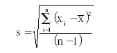
By making replicate analytical measurements, one can estimate the certainty of the analyte concentration using a computation of the confidence limits. As an example, given five replicate measurement results as: 5.30%, 5.44%, 5.78%, 5.00%, and 5.30%, the precision (or standard deviation) is computed using the following equation:

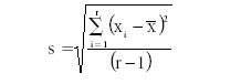
where s represents the precision, ∑ means summation of all the (x_i – X mean)² values, x_i is an individual replicate analytical result, x mean is the mean of the replicate results, and r is the total number of replicates included in the group (this is often represented as n). For the previous set of replicates, s = 0.282. The degrees of freedom are indicated by r – 1 = 4. If we want to calculate the 95% confidence level, we note that the t-value is 2.776. So the uncertainty (U) of our measurement result is calculated as

The example case results in an uncertainty range of 5.014 to 5.714 with an uncertainty interval of 0.7. Therefore, if we have a relatively unbiased analytical method, there is a 95% probability that our true analyte value lies between these upper and lower concentration limits.

Comparison Test for a Single Set of Measurements Versus a True Analytical Result

Let's start this discussion by assuming we have a known analytical value by artificially creating a standard sample using impossibly precise weighing and mixing methods so that the true analytical value is 5.2% analyte. We make one measurement and obtain a value of 5.7%. Then we refer to errors using statistical terms as follows:

Measured value: = 5.7%

"True" value: μ = 5.2%

Absolute error: Measured value – True value = 0.5%

Relative percent error: 0.5/5.2 × 100 = 9.6%

Then we recalibrate our instrumentation and obtain the results: 5.10, 5.20, 5.30, 5.10, and 5.00. Thus, our mean value (x mean) is 5.14.

Our precision as the standard deviation (s) of these five replicate measurements is calculated as 0.114 with n – 1 = 4 degrees of freedom. The t-value from the t table, α = 0.95, degrees of freedom as 4, is 2.776.

To determine if a specific test result is significantly different from the true or mean value, we use the test statistic (T_e):

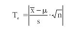
For this example, T_e = 1.177. We note that there is no significant difference in the measured value versus the expected or true value if T_e ≤ t-value. And there is a significant difference between the set of measured values and the true value if T_e ≥ t-value. We must then conclude here that there is no difference between the measured set of values and the true value, as 1.177 ≤ 2.776.

Comparison Test for Two Sets of Measurements

If we take two sets of five measurements using two calibrated instruments and the mean results are x mean₁ = 5.14 and x mean₂ = 5.16, we would like to know if the two sets of results are statistically identical. So we calculate the standard deviation for both sets and find s₁ = 0.114 and s₂ = 0.193. The pooled standard deviation s_1,2 = 0.079. The degrees of freedom in this case is n₁ – 1 equals 5 – 1 = 4. The t-value at α = 0.95, d.f. = 4, is 2.776.

To determine if one set of measurements is significantly different from the other set of measurements, we use the test statistic (T_e):

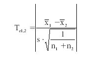
For this example, T_e1,2 = 0.398. So if there is no significant difference in the sets of measured values, we would expect T_e ≤ t-value, because 0.398 ≤ 2.776. And if there is a significant difference between the sets of measured values, we expect T_e ≥ t-value. We must conclude here that there is no difference between the sets of measured values.

Calculating the Number of Measurements Required to Establish a Mean Value (or Analytical Result) with a Prescribed Uncertainty (Accuracy)

If error is random and follows probabilistic (normally distributed) variance phenomena, we must be able to make additional measurements to reduce the measurement noise or variability. This is certainly true in the real world to some extent. Most of us with some basic statistical training will recall the concept of calculating the number of measurements required to establish a mean value (or analytical result) with a prescribed accuracy. For this calculation, one would designate the allowable error (e), and a probability (or risk) that a measured value (m) would be different by an amount (d).

We begin this estimate by computing the standard deviation of measurements. This is determined by first calculating the mean, then taking the difference of each control result from the mean, squaring that difference, dividing by n – 1, then taking the square root. All these operations are included in the equation:

where s represents the standard deviation; ∑ means summation of all the (x_i – X mean)² values; x_i is an individual control result; X mean is the mean of the control results; and n is the total number of control results included in the group.

If we were to follow a cookbook approach for computing the various parameters, we would proceed as follows:

• Compute an estimate of (s) for the method (see previous);

• Choose the allowable margin of error (d);

• Choose the probability level as alpha (α), as the risk that our measurement value (m) will be off by more than d;

• Determine the appropriate t-value for t_{1 – α/2} for n – 1 degrees of freedom.

• Finally the formula for n (the number of discrete measurements required) for a given uncertainty is as follows:

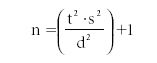
Problem Example: We want to learn the average value for the quantity of toluene in a test sample for a set of hydrocarbon mixtures.

s = 1, α = 0.95, d = 0.1. For this problem, t_{1 – α/2} = 1.96 (from t table), and thus n is computed as follows:

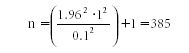
So if we take 385 measurements, we conclude with a 95% confidence that the true analyte value (mean value) will be between the average of the 385 results and 0.1, or X mean ± 0.1.

The Q-Test for Outliers (5–7)

We make five replicate measurements using an analytical method to calculate basic statistics regarding the method. Then we want to determine if a seemingly aberrant single result is indeed a statistical outlier. The five replicate measurements are: 5.30%, 5.44%, 5.78%, 5.00%, and 5.30%. The result we are concerned with is 6.0%. Is this result an outlier? To find out, we first calculate the absolute values of the individual deviations, as in Table I.

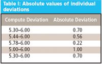
Table I: Absolute values of individual deviations

Thus the minimum deviation (D_Min) is 0.22; the maximum deviation 1.00; and the deviation range (R) is 1.00 – 0.22 = 0.78. We then calculate the Q-test value as Q_n using:

This results in the Q_n of 0.22/0.78 = 0.28 for n = 5.

Using the Q-value table (90% confidence level as Table II), we note that if Q_n ≤ Q-value, then the measurement is not an outlier. Conversely, if Q_n ≥ Q-value, then the measurement is an outlier.

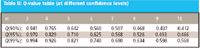
Table II: Q-value table (at different confidence levels)

So because 0.28 ≤ 0.642, this test value is not considered an outlier.

Summation of Variance from Several Data Sets

We sum the variance from several separate sets of data by computing the variance of each set of measurements; this is determined by first calculating the mean for each set, then taking the difference of each result from the mean, squaring that difference, and dividing by r – 1 where r is the number of replicates in each individual data set. All these operations are included in the following equation:

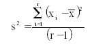
where s² represents the variance for each set; ∑ means summation of all the (x_i – X mean)² values; x_i is an individual result; X mean is the mean of each set of results; and r is the total number of results included in each set.

The pooled variance (s²_p) is given as

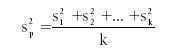
where s²_k represents the variance for each data set, and k is the total number of data sets included in the pooled group.

The pooled standard deviation σ_p is given as:

Jerome Workman, Jr. serves on the Editorial Advisory Board of Spectroscopy and is director of research and technology for the Molecular Spectroscopy & Microanalysis division of Thermo Fisher Scientific Inc. He can be reached by e-mail at: jerry.workman@thermofisher.com

Jerome Workman, Jr.

Howard Mark serves on the Editorial Advisory Board of Spectroscopy and runs a consulting service, Mark Electronics (Suffern, NY). He can be reached via e-mail at: hlmark@prodigy.net

Howard Mark

References

(1) J. Workman and H. Mark, Spectroscopy 21(9), 18–24 (2006).

(2) W. Horwitz, Anal. Chem. 54(1), 67A–76A (1982).

(3) P. Hall and B. Selinger, Anal. Chem. 61, 1465–1466 (1989).

(4) D. Rocke and S. Lorenzato, Technometrics 37(2), 176–184 (1995).

(5) J.C. Miller and J.N. Miller, Statistics for Analytical Chemistry (second edition) (Ellis Horwood, Upper Saddle River, New Jersey, 1992), pp. 63–64.

(6) W.J. Dixon and F.J. Massey, Jr., Introduction to Statistical Analysis (fourth edition), W.J. Dixon, Ed. (McGraw-Hill, New York, 1983), pp. 377, 548.

(7) D.B. Rohrabacher, Anal. Chem. 63, 139 (1991).