The Long, Complicated, Tedious, and Difficult Route to Principal Components: Part II
Howard Mark and Jerome Workman, Jr. continue their discussion of the derivation of the principal component algorithm using elementary algebra.

As we usually do, when we continue the discussion of a topic through more than one column, we continue the numbering of equations from where we left off. Therefore, while equation 1 is the same equation that we've seen before and therefore keeps its number, subsequent equations start with equation 11, since the last equation in the previous column (1) was number 10.

Jerome Workman, Jr.
We repeat our note that while our basic approach will avoid the use of matrices in the explanations, we will include the matrix expression corresponding to several of the results we derive. There are several reason for this, which were given in the previous column. It might not always be obvious that a given matrix expression is the decomposition of the algebraic equations stated. While it might not always be easy to go from the algebra to the matrix notation, it is always possible to confirm the correspondence by performing the specified matrix operations and seeing that the algebraic expression is recovered. For some of the more complex expressions, we present a demonstration of the equivalency in an appendix of the column.

Howard Mark
In this column, we will also start out by representing data arrays as matrices because that allows us to represent a whole array. However, we will not perform any computations on these matrices, although we will perform computations on the elements of the matrices when necessary, by using ordinary algebra.
That said, let us start with the data array, [X], as shown in equation 1:
Thus, the first piece of data in the array is a single spectrum consisting of m wavelengths:
Spectrum1 = [X 1,1 X1,2 X1,3 X1,4 . . . X 1,m ] [1a]
Similarly, the second row of the matrix [X] is
Spectrum2 = [X 2,1 X 2,2 X 2,3 X 2,4 . . . X 2,m ] [1b]
And so forth, for the n rows in the data matrix [X]:
Spectrumn = [X n,1 X n,2 X n,3 X n,4 . . . X n,m ] [1c]
All these spectra in the data set are combined into the single data matrix [X]:

Thus, the elements of the data matrix are designated by Xi,j, and the matrix has n rows and m columns. The columns represent different variables (for example, the absorbance at different wavelengths), and the rows represent spectra of different samples.
The goal is to find the function that, when multiplied by a suitable set of values and then subtracted row by row from the data matrix [X], is the best-fitting function. The "best-fitting" function in this sense means that the sum-squared differences (where the differences represent the error of the approximation) between the data matrix and the fitting function is the smallest possible value compared to any other function that could be used.
The situation is shown graphically in Figure 1, for two spectra, shown in black. The red curves in Figure 1 represent a principal component (shown in red); the same curve multiplied by two different scores so that they best approximate the two spectra. The error of the approximation is the difference between each spectrum and its approximation by the principal component, one of which is shown for each spectrum.
As we have seen in the previous column, the goal of minimizing the sum-squared error is the same as maximizing the variance accounted for by the fitting function. Because variance is taken around the mean of the data, it is convenient to subtract the mean spectrum from all spectra. As we saw, this simplifies the notation, because a quantity ΣX 2, for example, can now represent the variance directly, and, similarly, a quantity ΣX1X2 can represent a covariance directly.
As Figure 1 shows, the principal component loading, which is the label for the function that is used to fit the data, is the same for all spectra that are to be fitted. The difference between spectra is the coefficient that multiplies each loading. The function, or loading, is comprised of a set of values that differ from wavelength to wavelength, thus appearing as a spectrum itself. The function (which is the vector we call [L] to represent the fact that this function is what is called a "loading," in chemometrics-speak) will be designated by the vector:
[L] = [L1L2 L3 L4 . . . Lm] [11]
Then, for each row of the data matrix X, representing the several samples whose spectra make up [X], the function [L] will be multiplied by a different value of a weighting factor, or a "score" (as it is called, also in chemometrics-speak). Therefore, the set of scores (one for each row of the data matrix [X]) will be designated as the column vector [S]:
[S] = [S1 S2 S3 S4 . . . Sn ]T [12]
Thus, in order to determine the error of using the function [L] to give the first approximation to the first row of equation 1, we will have the array representing the approximation to the data:
S 1 [L 1 L 2 L 3 L 4 . . . L m ] = [S 1 L 1 S 1 L 2 S 1 L 3 S 1 L 4 ... S 1 L m ] [13a]
subtracted from it, term by term, where we see that each element of [L] is multiplied by the same score.
Similarly, row 2 will have the following array:
S2 [L 1 L2 L3 L 4 . . . L m ] = [S 2 L 1 S 2 L 2 S 2 L 3 S 2 L 4 ... S 2 L m ] [13b]
subtracted from it, term by term. This score, S 2 , is different than S 1 , the score for the first spectrum.
and so forth for every row, until finally we come to the last row, which will have the following expression subtracted from it, term by term:
S n [L 1 L 2 L 3 L 4 . . . L m ] = [S n L 1 S n L 2 S n L 3 S n L 4 . . . S n L m ] [13c]
(Note: the matrix equivalent of equation 13 is

(Exercise for the reader: perform the indicated matrix multiplication to demonstrate the equivalence to equation 13.)
The vector representing the loadings ([L]) is used to re-create the data array [X]. However, because the data could represent anything, it is clear that, with the possible exception of contrived test cases designed to make a point, no single function represented by any loading vector [L] could re-create all the rows of [X] simultaneously, because each row of [X] can represent a different function. Therefore, the loading [L], even after scaling it by the corresponding element of [S], is only an approximation to the data matrix. Thus, for example, the first row of the data matrix shown in equation 1 is approximated by the following product:
[S1 L 1 S1 L2 S1 L3 S1 L4 ... S1 Lm ] . . . [X1,1 X 1,2 X1,3 . . . X1,m ] [14]
However, an alternative method of indicating the approximate nature of equation 14 is traditionally used; the equality is kept, and the approximate nature of the equality is indicated by adding an "error" term to the equation:
[S1 L1 S1 L2 S1 L3 S1 L4 ... S1 Lm ] + [E] = [X1,1 X1,2 X1,3 . . . X1,m ] [15]
where [E] is the error vector [E 1 E2 E3 . . . Em ]; this allows us to keep the "equals" sign in the equation.
(Note: the matrix equivalent of equation 15 is:
S1 [L1 L2 L3 Lm] + [E 1E2 E3 Em ] = [X 1,1 X2,1 X3,1 Xm,1 ]
or, in short notation:
S1 [L] + [E] = [X])
This is all shown schematically in Figure 1. Figure 1 shows not only two of the spectra in a hypothetical data set and the principal components that estimate those spectra, but it also shows two of the error terms: the differences between the approximating principal component, and the actual data. Of course, what we are interested in here are all the error terms for all the spectra.
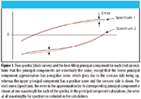
Figure 1
However, this is not the only relationship between the quantities S and L and the data matrix X. The scores, indicated by [S], are also functions of [L] and [X]. The values of the various Li comprising the vector [L] are normalized (or scaled) so that their standard deviation (and therefore their variance) equals unity. After this is done, the score corresponding to a row of the matrix [X] is computed from the following equation (we use row 1 as an example):

We will eventually make use of this relationship.
Going back to equation 15, we see from elementary algebra that the error for each term of the data matrix in equation 1 is the difference between the actual data point and the estimate from the principal component. Thus:
E1,1 = X1,1 – S1 L1
E1,2 = X1,2 – S 1 L2
E 1,3 = X1,3 – S1 L3
. . .
E1,m = X1,m – S 1 Lm
is the error vector for the first sample.
Similarly,
E2,1 = X 2,1 – S2 L1
E2,2 = X2,2 – S2 L2
E2,3 = X 2,3 – S2 L 3
. . .
E 2,m = X2,m – S2 Lm
is the error vector for the second sample, and so forth.
This can all be expressed by writing each error vector as a row in the following error matrix [E]:

This can also be put into the shorthand version of matrix notation (where the matrices [E], [X], [S] and [L] are as described in equation 10):

The distinguishing characteristic of principal components is that the loading is the "best possible" function that can re-create the data matrix [X]. "Best possible," in this sense, means that it is the function that can most closely reproduce the data matrix in the least squares sense. Therefore, the next task to find the values of the various Si,(i = 1,n) and L j,(j = 1,m) such that the sum of squares of the differences (or errors) in equation 15 is minimized. Because there is an error term for every wavelength and for each spectrum, to compute the necessary loadings and scores we first need to form the squares of all the terms (the terms at every wavelength for each spectrum), which we initially do in this simplistic form:
squared errors =

And then to get the sum squared errors (SSE) (which is what we intend to minimize), we need to add them all up:
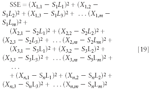
A shorthand way of presenting this is to express it in summation notation:

To generate the equations to solve and to allow us to find the values of S i and Li that satisfy equation 15, we execute the usual process of taking a derivative and setting that derivative equal to zero. We start by taking derivatives with respect to the several Sj. We start with a detailed examination of the derivative with respect to S1, and then the other derivatives can be handled similarly:
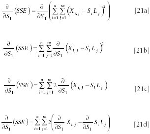
The data items are each constants; therefore, their derivatives with respect to S1 , and indeed with respect to all the Si , is zero. Therefore, equation 21d becomes:

The derivative of Si Lj depends upon the indices of the summations, or, at least, of the outer summation, over i. Because the derivative is being taken with respect to S1 , when i ≠ 1, the derivative is zero. When i = 1, the derivative is equal to the sum of the Lj.

By similar reasoning:

and so forth, for all values of 1 ≤ i ≤ n :

Setting each of these derivatives equal to zero, we obtain the following sets of equations:
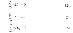
Finally, dividing both sides of each equation by –2, we obtain
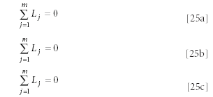
So we wind up with a set of n equations, all apparently identical. At this point we see that all of these equations have an identical, trivial, solution: that all the Lj are zero. That conclusion, however, is incorrect. To set all the Lj equal to zero would be valid only if the values for Lj were unconstrained. However, there is a constraint on the values of the Li . As we noted shortly after equation 15, the constraint is that the standard deviation of the Lj (and therefore their variance) is unity. Therefore, at least some of the Lj must be nonzero, and the trivial solution does not exist. We will pursue introducing the constraint in due course.
Another reason to conclude that at least some Lj are non-zero comes from the fact that the vector [L] is an estimator of the various values of Xi,j ; zero is prima facie not a good estimator of a set of functions. In fact, because each of the m equations represented by equations 25a–25c originated from a different Si, corresponding to a different row of the original data matrix, a better (in the least-squares sense, although equally trivial) solution is immediately obvious: set all the Lj equal to zero except for one of them (it doesn't matter which one), which can be set to any finite value (the ideal value would be that value that makes the variance of all the values of that column of [X] equal to unity). Then values of Si for the corresponding row of [X] can be found that, when multiplied by that value of Lj , cause the product Si Lj to equal the value of Xi,j . If this is done, then the difference between Si Lj and Xi,j will be zero, and therefore not contribute to the sum of squares of errors, making this sum of squares smaller than the sum of squares obtained when all the Lj are zero. This can be repeated, of course, for every row of [X], using the corresponding value of Si for that row, making all contributions of that variable to the sum of squares be zero. It is, however, also trivial in another sense: if all the errors were zero, then you could not reduce the error further, and therefore there would never be a need for any principal components beyond the first. Therefore, even though this solution is "better" (in the least-squares sense) than the original trivial solution, it is not the best possible solution, and certainly not the correct one, and so we must seek further.
Thus ends false start number 1.
Jerome Workman, Jr. serves on the Editorial Advisory Board of Spectroscopy and is with Luminous Medical, Inc. (Carlsbad, CA). He can be reached by e-mail at: jerry.workman@luminousmedical.com
Howard Mark serves on the Editorial Advisory Board of Spectroscopy and runs a consulting service, Mark Electronics (Suffern, NY). He can be reached via e-mail: hlmark@prodigy.net
References
(1) H. Mark and J. Workman, Spectroscopy 22(9), 20–29 (2007).
Note: The authors are proud to announce that 75 columns of "Chemometrics in Spectroscopy," including all columns from the May, 1993 issue to the February, 2007 issue, plus three others that have not yet appeared in Spectroscopy , have been collected and published in book form. For ordering information, please contact the author at hlmark@prodigy.net

LIBS Illuminates the Hidden Health Risks of Indoor Welding and Soldering
April 23rd 2025A new dual-spectroscopy approach reveals real-time pollution threats in indoor workspaces. Chinese researchers have pioneered the use of laser-induced breakdown spectroscopy (LIBS) and aerosol mass spectrometry to uncover and monitor harmful heavy metal and dust emissions from soldering and welding in real-time. These complementary tools offer a fast, accurate means to evaluate air quality threats in industrial and indoor environments—where people spend most of their time.
Smarter Sensors, Cleaner Earth Using AI and IoT for Pollution Monitoring
April 22nd 2025A global research team has detailed how smart sensors, artificial intelligence (AI), machine learning, and Internet of Things (IoT) technologies are transforming the detection and management of environmental pollutants. Their comprehensive review highlights how spectroscopy and sensor networks are now key tools in real-time pollution tracking.
New AI Strategy for Mycotoxin Detection in Cereal Grains
April 21st 2025Researchers from Jiangsu University and Zhejiang University of Water Resources and Electric Power have developed a transfer learning approach that significantly enhances the accuracy and adaptability of NIR spectroscopy models for detecting mycotoxins in cereals.