The Long, Complicated, Tedious, and Difficult Route to Principal Components: Part VI
This column is a continuation of the set we have been working on to explain and derive the equations behind principal components (1–5). As we usually do, when we continue the discussion of a topic through more than one column, we continue the numbering of equations from where we left off.

(Or, "When you're through reading this set you'll know why it's always done with matrices.")
This column is a continuation of the set we have been working on to explain and derive the equations behind principal components (1–5). As we usually do, when we continue the discussion of a topic through more than one column, we continue the numbering of equations from where we left off.

Howard Mark
We also repeat our note that while our basic approach will avoid the use of matrices in the explanations, we will include the matrix expression corresponding to several of the results we derive. There are several reasons for this, which were given in the previous columns. It might not always be obvious that a given matrix expression is the decomposition of the algebraic equations stated. While it might not always be easy to go from the algebra to the matrix notation, it is always possible to confirm the correspondence by performing the specified matrix operations and seeing that the algebraic expression is recovered. For some of the more complex expressions, we present a demonstration of the equivalency in an appendix of the column.

Jerome Workman
By the end of the last column, we showed that putting a constraint on the possible solutions to the problem of finding the least-square estimator to a set of data led to the inclusion of an extra variable in the variance-covariance matrix, which we called λ, representing the Lagrange multiplier. Expanding the determinant corresponding to the variance–covariance matrix gave a polynomial in the Lagrange multiplier; the roots of this polynomial give the values of λ that correspond to the nontrivial solutions of the original problem. However, that did not give us the function that actually corresponds to that value of λ, so we still have to determine the function corresponding to those roots, that is the least-square estimator. To do that, we need to develop the other solution to the problem of finding the solutions to the homogeneous equations (equations 46a–46c).
To determine the function, we note the following result we came up with, along the way to determining the value of λ. By the end of Part IV (4), we had come to the point of having derived the following set of equations, which we repeat here and for which we recall that the summations are taken over all the samples:

We begin by expanding the terms involving λ:
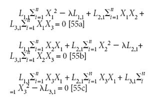
And then rearrange the equations:
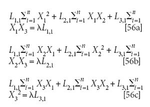
At this point we have no choice — we have to convert equations 56a–56c to matrix notation in order to see where we're going, when we get there:
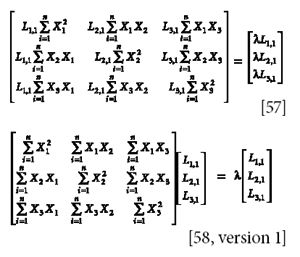
We will now write equation 58 out in shorthand matrix notation. We avoid using our usual "note" about it, which we normally use to indicate the conversion, for two reasons:
- Equation 58 is already in matrix notation, so we are not converting an algebraic-notation formula to matrix notation, which has been our usual practice when we insert the "notes."
- This particular matrix conversion is not incidental to the derivation as has been the usual case. It is the key part of it.
So equation 58 in shorthand matrix notation is

In this form, equation 58 might look familiar. If it doesn't look familiar, then perhaps converting the symbolism to a different set of symbols might make it more familiar.
So we replace [X] with H, λ with E, and [L] with ψ. Equation 58 now looks like this:

In this form, equation 58 is now instantly recognizable, from its use in quantum mechanics, as an eigenvalue equation. This, hopefully, should make clear why it was necessary to change algebraic equations 56a–56c into matrix equation 58; in addition to the recognition factor, the critical step is recognizing that the matrices in equation 58 represent a set of multivariate constructs and therefore have properties beyond the properties of the individual equations. Eigenvalues and eigenvectors are properties of the matrices [X] and [L]; they have no meaning with regard to the individual equations 56a–56c. Thus, the symbol E, standing for λ, is the eigenvalue of the system of equations; this is also the source of the characteristic equation, and of the identification of λ as the eigenvalues of equation 58. The corresponding eigenfunction, which is ψ, corresponding to [L], is the function that is the least-square estimator of the original data set, and must be obtained from the system of equations represented by equation 58.
Solutions to eigenvalue problems, like matrix inversions, are in the domain of computer science, not chemometrics. Therefore, at this point we pass on the details of solving the eigenvalue problem, as we did previously with the issue of matrix inversion (6), although later we will outline how one common procedure works.
However, we do note the following about this solution we noted before: that the characteristic equation for a data set containing n variables was of the form of a polynomial of degree n, and contained n coefficients for all the powers of λ. We also noted, however, that in order to generate the characteristic equation, the coefficients of λ came out of an expression requiring the evaluation of approximately n! determinants. For a typical data set of spectral data, containing, for instance, data at 100 or more wavelengths, the number of determinants to be evaluated would be (at least) 100! There isn't enough computer memory on earth, or enough time in the universe, to store all those intermediate values or evaluate the results.
So the conversion to an eigenvalue equation puts the theory in a form that provides a tractable solution to the original problem. Another key feature is that it provides the values not only for the eigenvalues (λ, in our principal component problem) but also the values for the rlements of the [L] array, the actual function that is the least-square estimator of the original data set. It also has the practical consequence of providing all these answers in the form of a solution that actually can be computed, on real computers and in reasonable amounts of time.
So to solve equation 58, we must find the values of λ and [L] that make the equation true. [L] is then the solution to equation 58 and also to the original problem. Because λ is a constant, λ[L] is a vector that is a simple multiple of [L] itself. In fact, we know how to find λ. We found it from our first attempt at solving the problem, using determinants. But knowing λ doesn't help us find [L], as we saw then. However, if we can find [L], then we can easily substitute it into equation 58, calculate λ, and see if the equation is then true.
The only caveat here is that eigenvalue solvers do not provide analytic algorithms (that is, there is no fixed algorithm corresponding to, for instance (to use the same comparison for our example case), matrix inversion algorithms, whereby a predetermined number of steps will convert the input data into the output results). Eigenvalue solvers work by approximation and iteration. In other words, we can make an initial guess as to the possible answer, that is, [L]. This guess doesn't have to be a very good guess. An array, for example, of all ones for the function can serve as an adequate starting guess. Let's call this guess [0L] = [1 1 1]T.
We then rewrite equation 58 as equation 59 and perform the computations needed to execute the matrix multiplication. This gives us a way to calculate (an approximation of) the elements of [L]:
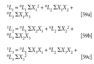
Then, directly from the definition given in the eigenvalue equation, we can expand the short form into the full expression of the matrices specified. Thus, if our initial guess is the approximation [0L], then multiplying [L] by [X] as indicated in equation 59 gives a new vector [1L] where each element of [L] is multiplied by the factors represented by the elements of the [X] matrix. Thus, by the rules of matrix multiplication:
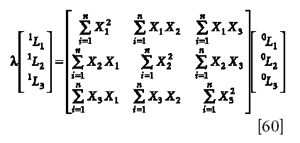
The two approximations to [L] are supposed to give the same values for [L], and also for λ. Therefore λ = 1L1/0L1 = 1L2/0L2 = 1L3/0L3. Then, according to equation 58, the computed values of 1L should be the same as the values of 0L (or some constant multiple of it). These considerations provide several ways to check whether we have found a value for [L] that satisfies the eigenvalue equation:
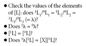
If one or more of these equations don't hold, that means that the approximation is not good enough; the algorithm has not converged on the correct function [L]. Normally, after the first round through the computation, none of these conditions will hold. However, the second (1L) approximation is a better approximation than the first one is. So on the first round, λ[L] ≠ [X] [L], but it has a better approximation to the correct [L] than the initial value (or guess, actually) was.
Therefore, we replace 0L with 1L and repeat the computation. Thus, if we iterate the computation, using each successive set of values for [L] to replace the previous one (2[L], 3[L], 4[L]. . . p[L]) as the next estimate, each value of [iL] is a better estimate of the correct value of [L] than the one before it.
Back in the algebraic world, this means that equation 59 can be written in a more general form, like this:
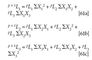
As the estimate gets better, the successive values of [L] become more nearly equal, until, at the point at which the computation has converged and [L] has attained the correct value, p – 1[L] = p [L]. In fact, at this point, when the computation has converged, all four conditions described earlier will hold, as they now satisfy equation 60.
It is normal, and recommended, that along the way some auxiliary computations are performed. In particular, because the various sums of squares and sums of cross-product terms in equation 59 can be, and often are, much larger or smaller than unity, the continued cycling of the [X] matrix through the algorithm can cause the computed values of the elements of the [L] matrix to become very large or very small. In principle, this should cause no problem, but in practice, it might happen that with enough cycling through the computation, the magnitude of the numbers can go beyond the limiting values that the computer can represent. To avoid this, the usual practice is that on each cycle through the computation, the [L] matrix is normalized to unit variance, by dividing each element by Σmi=1 Li2.
Once the computation has converged, the value of λ can be determined by dividing any given value of pLi by the corresponding value of p – 1 Li, before normalizing the value of p Li.
This gives us the value of the first principal component, which is the best possible least-squares estimator of data set that can be had based upon one function.
Because the first principal component is the best approximation to the data that can be achieved with a single function, then to further improve the approximation to the data, it is necessary to compute further principal components. Mathematically, one way this can be done is by adding more constraints to the problem: another Lagrange multiplier can be created (let's call it Φ), so that λ2 and Φ constitute a system of equation with two constraints, in addition to its being a least-squares estimator of the data set. One constraint is similar to the constraint for λ: 1 – L1,22 – L2,22 – L3,22 = 0. Note that the second subscript on L is now 2, indicating that we are now concerned with the second principal component. The second constraint is that the second loading (principal component) should be orthogonal to the first loading; this is expressed thusly: L1,1L1,2 + L2,1L2,2 + L3,1L3,2 = 0. The second constraint is added the same way as the first one: λ2 (1 – L1,22 – L2,22 – L3,22 ). The second constraint can be added directly, because the expression for the constraint already equals zero: Φ(L1,1L1,2 + L2,1L2,2 + L3,1L3,2). Then the same procedure of taking the derivatives and setting them equal to zero is applied, and the derivation continues from there.
In practice, the usual procedure is that the contribution of the first (or, in general, the current) principal component is removed from the dataset. Equation 16 (2) demonstrates how this is done. Basically, the idea is to compute the error term from fitting the first/current principal component to the data set. The steps needed are these:
- Normalize the principal component just computed, by dividing each element by Σmi=1 Li2, as described earlier.
- Compute the matrix product of the normalized principal component with the [X] matrix ([S] = [X][L]). This provides the set of scores ([S]) that is the contribution of that principal component to each data spectrum.
- For each sample, multiply the normalized principal component by the score for that sample; that is the contribution of that principal component to that spectrum.
- For each spectrum, subtract that contribution due to the first principal component, wavelength by wavelength, from the corresponding spectrum.
The principal component calculated will be principal component 2; the function that is the leastsquare fitting function to the error terms remaining from the first principal component. The two functions, together, will account for more variance from the original data set than any two functions, of any sort, can.
Summary
We have now plowed our way through considerable mathematical territory, while deliberately taking two dead-end side trips. In the process, we demonstrated the following:
- We showed algebraically that the maximum variance functions describing a set of data are the least squares function that approximate that data set.
- We showed algebraically that the least squares solution is not simply a collection of multiple univariate solutions, in which the least squares value at each individual wavelength (or other variable), but requires the full variance–covariance matrix to properly describe the least-squares nature of the problem.
- We showed algebraically that even so, the least-squares formulation of the problem results in a trivial solution, unless somehow you can impose a constraint on the solutions so that nontrivial solutions can be found.
- We showed algebraically that the method of Lagrange multipliers is a way to impose the necessary constraint.
- We showed that finding the least square solutions required the use of derivatives, because the extremum is found by setting the derivative equal to zero. This result comes from elementary calculus, our only departure from a purely algebraic approach.
- We then showed algebraically how the Lagrange multiplier comes out of the equations as a polynomial (called the "characteristic equation"); therefore, there are as many solutions to the problem as there are roots to the polynomial. These multiple roots correspond to the multiple principal components we can calculate.
- To calculate the functions corresponding to the roots of the characteristic equation, which are the functions that are the least-squares fit to the original data set, we recast the equations into the form of an eigenvalue equation. From this we found that the eigenvalue corresponds to the root of the characteristic equation, and the eigenfunction is the function that is actually the least-square estimators of the original data set.
- Then, we subtract the contribution of the given principal component from the data set, and do the whole procedure all over again, to find the next principal component. Iterate until you've approximated the data set to a sufficient degree of accuracy, or run out of time, money, computer capacity, or patience.
Thus ends the story of the long, complicated, tedious, and difficult route to principal components. That's why it took us six of our columns to explicate it all.
And THAT'S why principal components are always done with matrices!
However, don't miss the coda we will present in our next installment.
References
(1) H. Mark and J. Workman, Spectroscopy 22(9), 20–29 (2007).
(2) H. Mark and J. Workman, Spectroscopy 23(2), 30–37 (2008).
(3) H. Mark and J. Workman, Spectroscopy 23(5), 14–17 (2008).
(4) H. Mark and J. Workman, Spectroscopy 23(6), 22–24 (2008).
(5) H. Mark and J. Workman, Spectroscopy 23(10), 24–29 (2008).
(6) H. Mark and J. Workman, Spectroscopy 21(6), 34–36 (2006).
Howard Mark serves on the Editorial Advisory Board of Spectroscopy and runs a consulting service, Mark Electronics (Suffern, NY). He can be reached via e-mail: hlmark@prodigy.net
Jerome Workman, Jr. serves on the Editorial Advisory Board of Spectroscopy and is currently with Luminous Medical, Inc., a company dedicated to providing automated glucose management systems to empower health care professionals.

LIBS Illuminates the Hidden Health Risks of Indoor Welding and Soldering
April 23rd 2025A new dual-spectroscopy approach reveals real-time pollution threats in indoor workspaces. Chinese researchers have pioneered the use of laser-induced breakdown spectroscopy (LIBS) and aerosol mass spectrometry to uncover and monitor harmful heavy metal and dust emissions from soldering and welding in real-time. These complementary tools offer a fast, accurate means to evaluate air quality threats in industrial and indoor environments—where people spend most of their time.
Smarter Sensors, Cleaner Earth Using AI and IoT for Pollution Monitoring
April 22nd 2025A global research team has detailed how smart sensors, artificial intelligence (AI), machine learning, and Internet of Things (IoT) technologies are transforming the detection and management of environmental pollutants. Their comprehensive review highlights how spectroscopy and sensor networks are now key tools in real-time pollution tracking.
New AI Strategy for Mycotoxin Detection in Cereal Grains
April 21st 2025Researchers from Jiangsu University and Zhejiang University of Water Resources and Electric Power have developed a transfer learning approach that significantly enhances the accuracy and adaptability of NIR spectroscopy models for detecting mycotoxins in cereals.