Quantitative Mass Spectrometry Part IV: Deviations from Linearity
In the fourth part of a five-part series, columnist Ken Busch discusses factors that might cause deviation from linearity at the upper and lower limits of a calibration curve.

In a quantitative analysis using values measured with mass spectrometry (MS) — usually values associated with ion intensities — a nonlinear regression (weighted or nonweighted) might model the proportionality between measured instrument response and sample amount more accurately. We begin by considering general factors that might cause deviation from linearity at the upper and lower limits of a calibration curve. Recall that in quantitative spectrophotometry (in which a linear relationship is established by the equation A = εbc, where A is the measured absorbance, ε the molar extinction coefficient, b the path cell length, and c the sample concentration), the phenomenon of self-absorbance is presented as one of many reasons for a "deviation from Beer's law," resulting in a "turning over" of the measured absorbance curve at higher sample concentrations (Figure 1). In the simplest of terms, this phenomenon results when sample molecules no longer interact independently with the incident light beam. For some molecules in solution, the intensity of the incident light has been attenuated already by prior interaction with other sample molecules in the cell. Beer's law and its deviations is a popular undergraduate laboratory experiment, and for an intermittently tongue-in-cheek discussion of Beer's law as applied to the analysis of dark beers, see reference 1. Statistical and nonlinear methods have been developed over many years to extend the useful range of quantitation using Beer's law.

Kenneth L. Busch
Analogous deviations from linearity of a calibration line can occur in quantitative MS. For example, a space charge effect related to the absolute number of ions in an ion source, or stored within an ion trap, can act to decrease the intensity of the expected signal. The "self-chemical ionization" phenomenon (again in ion traps) can transfer ion intensity from the molecular ion to the protonated molecule at higher sample concentrations. The central tenet of these "deviations" is that each sample molecule no longer acts independently of the presence of all the others. The performance of ionization sources, especially as they become smaller, can become exquisitely dependent upon the absolute amount of sample present. Depending upon the ion chemistry of the sample, the ion intensities chosen for measurement, and the matrix, the desired simple linear relationship between the amount of sample and a measured ion intensity value can become complicated. For example, and especially for lower mass ions, multiple paths of formation for any one particular ion can be implicated. Additionally, at higher concentrations of sample, multiple isobaric ion species at the same nominal ion mass can appear and overlap, especially as resolution requirements are relaxed in a quest for higher signal levels. Interestingly, in the case of matrix effects, higher concentrations might result in a deviation in measured signal intensity in either direction, depending upon a myriad of unexplored details. Sometimes these multiple factors can conveniently offset each other to maintain an apparent linearity. But most often, higher sample concentrations cause some decrease in the expected measured signal intensity. Remember, too, that an ionization source, and the extraction of ions from it, represents a specific snapshot of ions formed within a certain time window. Higher sample concentrations sometimes invoke complicated kinetics and higher order reactions that depend upon sample concentrations. Fascinating chemistry can be found there. Stressed analysts and us old folk usually prefer the predictable comfort of the linear range.
At the lower end of the calibration curve in spectrophotometry, to reuse the example, deviations from Beer's law again are due to a number of factors, including (at the lowest levels) random detector noise. However, in quantitative MS, analysts seldom make measurements at or near the instrumental noise limit. Instead, other factors conspire to establish a lower limit of detection (LOD) usually delimited by matrix effects and chemical noise. For example, one oft-encountered phenomenon of lower-limit operation is that no measured response is seen until sample concentration reaches a certain minimum value. This phenomenon usually is attributed to unspecified sample losses. In the vernacular, we refer to "feeding the system." Mass spectrometrists, of course, are required by revered spectroscopic fraternity tradition to attribute such losses as occurring solely in the chromatographic column that precedes the mass spectrometer. A gas chromatography (GC) column, for example, along with its associated injection port, transfer lines, and connections, might contain a variety of active sites that can seemingly irreversibly absorb small amounts of sample. In GC, a carrier compound is sometimes used to minimize this sample loss and extend the linear proportionality of response to lower values. Of course, the sample loss problem also exists for components of the mass spectrometer. It is usually limited to the sample introduction system and ionization source components of the mass spectrometer, since system operation past that point usually involves ions held in vacuum, far removed from active sites in the physical environment. Note that if the effect of active sites, wherever they might be found, is significant, the order in which standards are run might create an apparently variable instrument response. As an example, results at the end of the day might seem to reflect a higher "sensitivity" than those at the beginning of a series of runs. Unexplained but repetitive trends in analytical results can be the result of such unappreciated phenomena.
The more complicated the overall analytical schema, including multiple stages of MS as in MS-MS, the more likely that the individual contributions to variance are not assignable. However, even if the source of variance is unknown, if it is predictable, then the contribution can be modeled and the quantitative analysis can proceed nevertheless. A mathematical model that best fits observed data can be described mathematically as exponential, logarithmic, Gaussian, or others, or combinations thereof. An analyst might seek a subsequent linearization of the data (as in the Beer's law relationship described earlier), but should recognize that this process itself affects any subsequent treatment of errors. A direct nonlinear (and sometimes weighted) model can be used to "fit" the data directly, and the requisite mathematics is often within the scope of the commercial spreadsheet or simple data analysis programs on a personal computer. Remember that the mathematical model is only that — it is not an explanation of underlying molecular reactions and ionic dynamics, even if the fit to the data is excellent. Nonlinear regression is described in several classic textbooks (2,3) and is a component of several free and commercial statistics software packages (4). The current column is a simplified exposition of a complex topic covered in more detail in those resources.
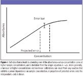
Figure 1
Consider first the shape of the calibration curve illustrated in Figure 1, in which the measured instrument response "turns over" at higher sample concentrations. As noted, a curve of this shape can be found in quantitative spectrophotometry, but it also can be seen in MS when, for example, the intensity of a measured ion (or ions) is reduced by a reaction that exhibits a power dependence on sample concentration. As the curve bends over, the projection of error from the y axis onto the x axis grows, as shown in the figure. In other words, in determining the sample concentration from the calibration, the range of possible answers (with the same analytical uncertainty) grows. This seems especially counterintuitive, as it would seem that a higher measured signal level should lead to greater accuracy. Now consider the alternative response curve shown in Figure 2, with the observed instrumental response at higher concentrations arcing in the other direction. While such a situation is encountered more rarely, it can be encountered in an MS quantitation when the intensity of a molecular ion is monitored, and a higher sample concentration leads to a situation in which internal energy in that ion is relaxed (as in collisional quenching). At first, we might think this might be desirable in that a magnified proportionality between response and sample amount would lead to a better ability to determine the sample concentration. The expected random errors in response measurement project onto a smaller breadth of possible answers on the x axis. What might occur instead, however, is that the lack of true independence in the creation of standards becomes evident. That is, an error associated with the creation of standards of "known" concentration amplifies the variations seen in the measured instrument responses. Perhaps most undesirable, at least on first examination, is a situation in which a complex curve is seen. Even this situation can be modeled accurately with statistics, and errors on both axes examined.
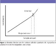
Figure 2
What is a nonlinear regression? Simply put, the parameter or parameters that determine the measured response do not occur as linear combinations of independent variables. Examples include the exponential or logarithmic functions that link instrument response to amount of sample. But S-shaped curves, and Gaussian and Lorentzian functions, are also nonlinear fits to data. If the model is physically realistic, the match between experimentally measured data and model can be extraordinary. Note that this quantified curve fit is different from a similarly shaped curve (such as Figure 1) in which deviations from the assumed linear model are apparent. A nonlinear regression can be appropriate when the number of significant independent variables changes as the concentration range is traversed. Again, limitation of the analysis to a more constricted linear range dependent on only one variable simplifies the best-fit mathematics, but the broader analytical range can still be modeled adequately with nonlinear regression methods.
Most nonlinear regressions are accomplished mathematically without a weighting scheme. As in the linear least-squares regression, the mathematical program minimizes the sum of the squared vertical distances of the model curve from the actually measured values. The assumption in this treatment is that factors that lead to scatter in the experimentally measured values are equal at all points along the curve. This assumption might be realistic over a single decade of sample concentrations, but it becomes suspect as the breadth of the calibration curve extends to two or three orders of magnitude. As a matter of experience, the observed variation in repetitive measurements of an experimental intensity for a single independent variable value often is related to the absolute values themselves. Simply stated, the observed range of errors is proportional to the value, as illustrated conceptually in Figure 3. Statistical tests can be used to establish the extent of this variance.
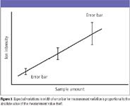
Figure 3
What is the practical consequence of this dependence? One consequence is that the regression analysis is best accomplished with a weighting method. The 1/y2 weighting minimizes the sum of the squared values for relative distances of experimental points from the best-fit curve. This weighting method is appropriate when, as shown in Figure 3, the expected errors are higher at higher measured values. In this instance, although the absolute size of the error bar at higher y values increases, the relative value ([range of errors in y]/y) is assumed to remain constant. Again, this is a mathematical assumption, and not necessarily the real observed or real physical model. In situations in which another function describes the distribution of error bar widths, a different weighting scheme might be appropriate (the 1/y weighting scheme is an example). The 1/y2 weighting is the most commonly found in nonlinear regression used in quantitative MS.
For example, Uran and colleagues (5) recently described a liquid chromatography–electrospray ionization MS (LC–ESI-MS) method for the quantitation of 13 C-pyruvate and 13 C-lactate in dog blood after derivatization of these analytes with 3-nitrophenyl hydrazine. A response range across three orders of magnitude was determined using internal standards and a nonlinear equation of the form y = a + bx + cx2 and a weighting factor of 1/y2. This example illustrates the use of a nonlinear regression analysis in a classic quantitative MS analysis based upon the proportionality between measured instrument response and the amount of the targeted compound. Moreover, the method is applied to a situation in which MS is uniquely capable — the analysis of a nonradioactive isotopically labeled sample. MS is replete with examples in which nonlinear regression methods are used at some other point in the measurement, perhaps several steps removed from a quantitation goal. For example, Daikoku and colleagues (6) successfully used energy-resolved MS in an ion trap to differentiate between 16 structural isomers of disaccharides. Sigmoidal plots for the decay of the sodiated parent ion intensity and the growth of a characteristic product ion intensity were recorded as a function of ion collision energy, with the collision energy established by variation of the rf amplitude applied to the end-cap electrode of an ion-trap mass spectrometer. Data collected in a number of data sets (between 13 and 21, depending upon the isomers) were treated using a nonlinear regression analysis to accurately model the growth and decay curves. Once this was completed, parameters used to describe the curves were displayed in a scatter plot. A visual comparison of the growth and decay curves served to differentiate many of the isomers. However, use of a nonlinear regression and a statistical evaluation of the scatter plot (which takes into consideration the confidence levels for each set of parameters) allowed all 16 isomers to be differentiated clearly. This sophisticated data treatment is predicated upon the fact that the parent ions are created in a standard manner that can be duplicated. Thus, the challenge underlying such a sophisticated analysis extends to our ability to control the ionization process through which ions are formed and sampled, as well as our ability to maintain our instruments in a stable and well-defined state.
We note that recent texts on quantitative MS are available to the analyst (7–9). These texts boldly advance into the full world of quantitative MS and include details on such topics as homoscedastic and heteroscedastic models, and the proper statistical models for each of these two different types of variance. These models form the basis of the weighting schemes discussed earlier. We have studiously limited ourselves to the nonmathematical models in this column. Additionally, the role of quantitative MS in proteomics recently has been reviewed separately (10). Each of the methods used in quantitative MS must derive from a sound and thorough understanding of statistics, and a consensus set of definitions for the community. In this regard, the overview article of Mark (11) on testing the linearity of an analytical method is highly recommended.
In the final installment of this series, we will describe a few examples of quantitative MS well removed from the classic linear calibration to determine the amount of sample. Such examples are drawn from topics as diverse as ion kinetics and heuristics. Additionally, a few graphical examples of quantitation will be drawn from the recent published literature. These examples will be anonymous, and will be chosen because they can leave the reader a bit skeptical, or wishing for additional data. Egregious errors in quantitative MS seldom survive peer review of results for validity or publication. However, at the same time, reviewers seldom have time to explore voluminous data in depth to confirm the validity of the statistical methods applied. Examples that leave us a bit unsure or unconvinced remind us all to make the full appropriate effort in both data collection and presentation.
Kenneth L. Busch asserts that quantitative MS is one of the top 10 (±1) achievements of modern analytical science. Unrelenting pressure to provide answers more quickly at lower limits of detection for samples drawn from more complex matrices distracts attention from new ion chemistries and new informatics that will develop over the next decades. Views in this column are those of the author and not the National Science Foundation. KLB can be reached at wyvernassoc@yahoo.com
References
(1) brewingtechniques.com/brewingtechniques/beerslaw/index.html
(2) G.A.F. Seber and C.J. Wild, Nonlinear Regression (John Wiley and Sons, New York, 1989).
(3) R.M. Bethea, B.S. Duran, and T.L. Bouillion, Statistical Methods for Engineers and Scientists (Marcel Dekker, New York, 1985).
(4) "Fitting Models to Biological Data Using Linear and Nonlinear Regression," April 2003, available at www.graphpad.com.
(5) S. Uran, K.E. Landmark, G. Hjellum, and T. Skotland, J. Pharm. Biomed. Anal. 44(4), 947–954 (2007).
(6) S. Daikoku, T. Ako, R. Kato, I. Ohtsuka, and O. Kanie, J. Am. Soc. Mass Spectrom. 18(10), 1873–1879 (2007).
(7) M.W. Duncan, P.J. Gale, and A.L. Yergey, The Principles of Quantitative Mass Spectrometry (Rockpool Productions, Denver, Colorado, 2006).
(8) I. Lavagnini, F. Magno, R. Seraglia, and P. Traldi, Quantitative Applications of Mass Spectrometry (John Wiley, New York, 2006).
(9) R.K. Boyd, R. Bethem, and C. Basic, Trace Quantitative Analysis by Mass Spectrometry (John Wiley, New York, 2008).
(10) M. Bantscheff, M. Schirle, G. Sweetman, J. Rick, and B. Kuster, Anal. Bioanal. Chem. 389(4), 1017–1031 (2007).
(11) H. Mark, J. Pharm. Biomed. Anal. 33, 7–20 (2003).

High-Speed Laser MS for Precise, Prep-Free Environmental Particle Tracking
April 21st 2025Scientists at Oak Ridge National Laboratory have demonstrated that a fast, laser-based mass spectrometry method—LA-ICP-TOF-MS—can accurately detect and identify airborne environmental particles, including toxic metal particles like ruthenium, without the need for complex sample preparation. The work offers a breakthrough in rapid, high-resolution analysis of environmental pollutants.
The Fundamental Role of Advanced Hyphenated Techniques in Lithium-Ion Battery Research
December 4th 2024Spectroscopy spoke with Uwe Karst, a full professor at the University of Münster in the Institute of Inorganic and Analytical Chemistry, to discuss his research on hyphenated analytical techniques in battery research.
Mass Spectrometry for Forensic Analysis: An Interview with Glen Jackson
November 27th 2024As part of “The Future of Forensic Analysis” content series, Spectroscopy sat down with Glen P. Jackson of West Virginia University to talk about the historical development of mass spectrometry in forensic analysis.
Detecting Cancer Biomarkers in Canines: An Interview with Landulfo Silveira Jr.
November 5th 2024Spectroscopy sat down with Landulfo Silveira Jr. of Universidade Anhembi Morumbi-UAM and Center for Innovation, Technology and Education-CITÉ (São Paulo, Brazil) to talk about his team’s latest research using Raman spectroscopy to detect biomarkers of cancer in canine sera.