Calibration Transfer

The results we found from our previous subseries about classical least squares analysis provides the mechanism for understanding when and why calibration transfer can be done easily or when it will be difficult. Those results also provide a basis for a modified understanding of what calibration transfer means and how we can tell whether or not such a transfer can be performed, for any given analysis.

Calibration transfer is an important and popular topic for both the science and practical applications of near-infrared (NIR) spectroscopy. However, there is no consensus on the meaning of the term, and any claims of calibration transfer may be well nigh meaningless in a scientific sense, despite its practical importance. We propose a definition, and a method of evaluating calibration transfer, based on our recent discoveries about the nature of light absorbance in spectroscopic analysis.

Jerome Workman, Jr.

Before we continue, therefore, let's recap the key findings of our previous column (1) and what the new discoveries were:

1) Different measures of concentration commonly used for reference laboratory values for NIR calibrations do not (repeat not) have a one-to-one correspondence (that is, they do not form a bijective function) with each other. An important example is the weight fractions of the components in a mixture compared to the volume fractions of those components.

Howard Mark

2) The different concentration measures are not linearly related to each other.

3) The NIR absorbances, operative for the spectral values used in calibrations, are in fact related to the volume fractions of the mixture components.

4) The lack of bijectivity of point 1 and the nonlinearity of point 2 have nothing to do with the spectroscopy.

It took considerable head-scratching, but eventually the realization dawned that the underlying properties leading to both characteristics are purely the physical chemistry of the mixtures. This is further illustrated in Figure 1, which shows the relationships between weight fractions and volume fractions for the set of mixtures of toluene, dichloromethane, and n-heptane, as examined in our previous column (1).

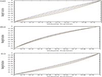
Figure 1: Weight fractions versus volume fractions of (a) toluene, (b) dichloromethane, and (c) n-heptane in ternary mixtures of the three compounds.

These properties of mixtures shed much light (no pun intended) on the behavior of mixtures and on the effect of that behavior on the various calibration algorithms that we apply. There are many implications and ramifications of the new knowledge we have gained, which are touched upon in another publication (2). Here, we discuss the effects of these properties on the behavior of data when we perform calibration transfer exercises.

"Calibration transfer" has been a buzzword in NIR spectroscopy for as long as NIR has been practiced. Other labels have been used over the years, such as "universal calibration," but the concept was the same: to create a calibration model on one instrument and apply it to samples measured on a different instrument. However, there were never any specifications to describe, or even define, what we meant by calibration transfer. No objective criteria were ever set up, by which we could ever know whether we had, in fact, successfully transferred a calibration, or what results can be expected from applying a transferred calibration to routine analysis.

In place of a formal definition, an empirical procedure has been used, which therefore has also been serving as a de facto definition. The procedure is to attempt transferring a calibration from one instrument to another, and then testing whether the transfer has succeeded. "Success" is determined by the agreement between the accuracy from the analyses on the "parent" instrument (also called the "master") instrument with the accuracy of the analytical results on the second instrument (usually called the "child" or "slave" instrument). Samples different than the ones used for calibration are usually measured on the child unit in order to simultaneously validate the calibration through the use of the separate sample set.

However, this empirical procedure conflates (the proper statistical term is "confounds") the issue of calibration transfer with the issue of whether the original calibration is any good to start with, whether the new sample set used to test the transfer capability is itself a proper set, and also whether the reference laboratory values are appropriate and have the same accuracy as the ones used for the calibration sample set. In principle, a true calibration transfer procedure should provide the same analytical performance on the two instruments, whether that performance is good or bad. With the current state of affairs, if we get good (accurate) performance on both instruments then that constitutes evidence that all is well. On the other hand, if we get good (accurate) performance on the parent instrument but poor performance on the child instrument, we have no information as to whether that is because of the calibration being nontransferable, a defect in the child instrument, an improper set of test samples, or a set of samples for the child instrument that has poor reference laboratory values.

Our previous exposition of the behavior of classical least squares (CLS) and the results from applying it to data was unfortunately never completed. We do hope to eventually publish "the rest of the story" (with all respect to Paul Harvey), but for now we will jump ahead of that full exposition to make use of some of the results and learn what they tell us about the behavior of data for calibration transfer.

Experimental

The data used were taken from the 2002 International Diffuse Reflectance Conference (IDRC, Chambersburg, Pennsylvania) as the dataset for the "Software Shootout" at that conference. It was made publicly available and is described and can be downloaded from the following web page: http://www.idrc-chambersburg.org/ss20022012.html.

The contributors of the "Software Shootout" dataset also published their results from it (3); the publication also includes a more detailed description of the data.

More details concerning the instrumentation, sample preparation, and measurement procedures can also be found in the above-cited article (3). In this article, we concentrate our attention on the results from the 155 pilot plant calibration samples. Suffice it to say, for now, that we found equivalent results from the other two data sets included in that shootout data.

For the sake of completeness we note that for the purposes of the shootout, the instruments were arbitrarily designated unit 1 and unit 2. All our calibrations were performed on data from unit 1 and the models were used to predict corresponding measurements from unit 2.

Results

Our attention was particularly drawn to the behavior of this shootout sample set when we noticed the outliers in the calibration and prediction plots.

We performed several calibrations, using various transformations of data from unit 1 and, as described above, the model developed was used to predict the data from unit 2. The plot in Figure 2a shows the predicted-versus reference values for the calibration samples using a partial least squares (PLS) model with eight factors. Figure 2b shows the corresponding prediction results from instrument 2. Similarly, Figures 3a and 3b show the instrument versus reference values plots for a model using a different data transform. The readings considered outliers are circled.

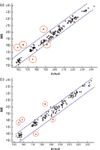
Figure 2: Plot of actual (that is, reference laboratory) values versus predicted (that is, from the model) values. For the plots in this figure, the data transform was absorption to reflection followed by normalization, and the algorithm was PLS-1, using eight factors. (a) The calibration results from instrument 1. (b) The prediction results from instrument 2.

It should be noted that the pattern of outliers is the same for all four plots: two models on each of the two instruments. We performed a good number of other calibrations, using different data transforms, different transform parameters (for example, number of data points used for smoothing, or the gap for a derivative), different calibration algorithms, and different numbers of factors (or wavelengths, in the case of multiple linear regression [MLR]). In the interest of saving space we forbear to present all these plots, it suffices to note here that for all calibrations and predictions, the same pattern of outliers were observed.

In the software shootout, most if not all, of the contestants obtained plots similar to the one shown in Figures 2 and 3. Because the goal of the shootout was to optimize the prediction of the analyte value (the active pharmaceutical ingredient [API] in a pharmaceutical product), most of the contestants in the shootout either deleted the outlier samples or tried to accommodate them with more PLS factors or different data transformations.

Figure 3: Plot of actual values versus predicted values. For the plots in this figure, the data transform was absorption to reflection followed by normalization, the algorithm was PLS-1, using five factors. (a) The calibration results from instrument 1. (b) The prediction results from instrument 2.

However, we noted another curious fact about the outliers: The same ones appeared on both instruments. It is clear from the plots of Figure 2, for example, that the outlier points seem to come in the same places in both sets of data. More careful inspection, which involved looking individually at which samples were the outliers, revealed that the same actual samples gave the same outliers in the data sets from both units.

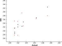
Figure 4: Results from the two instruments plotted on the same axes using different colors. Values from unit 1 are shown in black and from unit 2 in red. Only the samples at the upper end of the range are plotted because otherwise, the middle of the graph was too crowded with data points to determine what was happening. Therefore, only the results from the highest-value samples are presented here.

At this point, it appeared that no matter what calibration conditions were used, the same outliers appeared on both instruments, and in the same places. Several questions then arose: What about the rest of the samples? How were they behaving in all this? Did they also fall in the same places for all the different conditions?

Figure 4 shows the results, using no data transform and a five-factor PLS model, from unit 1 and unit 2 plotted on the same axes, against the reference laboratory results. The two instruments' results are distinguished by their colors. In Figure 4, we can see how the results from the two instruments are paired up, showing that they are both providing the same predicted values.

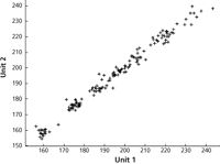
Figure 5: Spectroscopically predicted values from unit 1 versus the corresponding values from unit 2, with no data transformation and a five-factor PLS model.

To examine the behavior of the rest of the samples, which constituted the majority of the dataset, a different type of plot was needed. Figure 5 illustrates that the results from the two instruments are in close agreement with each other. We also note that there are no readings that stand out as outliers in this plot. What appear to be matching outliers in the previous plots are the result of the two instruments' readings agreeing with each other (parenthetically we also note, therefore, that the outliers in the previous plots appear to point a finger at the reference laboratory results as the cause). To demonstrate that these results are not unique, Figure 6 presents similar results using a different data transform, one chosen at quasi-random from among the many that were tried, in this case multiplicative scatter correction (MSC) plus the second derivative data transformations and a four-wavelength MLR model.

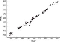
Figure 6: Spectroscopically predicted values from unit 1 versus the corresponding values from unit 2, with MSC plus second derivative data transformation and a four-wavelength MLR model.

Having performed all these various calibrations (and others, not shown) it became quite clear that fiddling with the calibration conditions made, at most, minor differences in the behavior of the results, or with the ability of the instruments to agree with each other. We summarize this behavior in Table I. In Table I we see that the instruments agree with each other at least as well as either one agrees with the reference laboratory (better, if the correlation coefficient is used as the criterion).

Table I: Results obtained using the actual reference laboratory values

One question still that remained to be answered, however, was whether the behavior of the data was due to some peculiarity of the particular set of readings we were dealing with, especially the reference values.

To investigate this question, the reference laboratory values were replaced with random numbers. Because the samples that were measured on the two instruments were aliquots from the same samples, the same random number was used as the replacement for the corresponding reference value on both instruments. Calibration on data from unit 1 and prediction of the data from unit 2 were then performed in the usual manner. These results are shown in Figure 7. We can see that there is very little, if any, relationship between the (random) reference laboratory values and the instrument results, as we would expect.

Table II: Results obtained using random numbers for the "reference" values

Similarly, as we did before, we present a graph of the results from instrument 1 plotted versus the results from instrument 2; this is shown in Figure 8. The numerical value for the correspondence between the two instruments' results is shown in Table II. Both the graphical and numerical results demonstrate that the instruments agree with each other very well, in fact considerably better than they agree with the reference laboratory results. Here again, different data transformations as well as different calibration algorithms were tried, with essentially the same results in all cases.

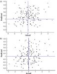
Figure 7: Spectroscopically predicted calibration (a) values from unit 1 versus the corresponding random "reference laboratory" values, with MSC plus second derivative data transformation and a four-wavelength MLR model. (a) The calibration results from instrument 1. (b) Prediction results from instrument 2, using a calibration developed from random "reference laboratory" values.

Table II also presents the numerical values corresponding to these graphs. Because the random numbers do not correspond to any actual constituent values, we ignore those statistics that depend on actual physical values for the errors of the analysis, that is, the standard error of the estimate (SEE) and the standard error of prediction (SEP); and of necessity, therefore, we present only the correlation coefficients.

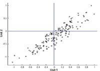
Figure 8: Values predicted by instrument 1 versus values predicted by instrument 2 when the simulated "reference laboratory" values were random numbers.

Discussion

Thus, we see that regardless of the data transformation or the calibration algorithm used, the predicted values depended only on the composition of the samples, mostly independently of even the well-known "particle size" effects. A brief summary of these results was previously published in Spectroscopy (4).

At that time, however, we had no idea what was causing this behavior and that the instruments would agree with each other better than they did with the reference laboratory, even when the "reference laboratory" was a set of random numbers. The only lesson learned from these findings was that ". . . you should not use NIR as a reference laboratory method for calibrating another NIR instrument, since NIR agrees with NIR regardless of the agreement with anything else" (4).

More recently, however, some important information about the behavior of spectroscopic measurements was developed, this was published in Applied Spectroscopy (2) as well as the previous series in Spectroscopy, of which reference 1 is the predecessor of this column. This article provides a mechanistic explanation for the effects seen, as will soon be demonstrated.

Here are the key findings that emerged from the previous study:

• Contrary to the previously held assumption that different measures of concentration are equivalent except for scaling factors, different concentration measures behave differently as the sample composition changes. The relationships between different concentration measures are not only nonlinear, the relationship between different measures is not necessarily unique; a given value of concentration by one measure can correspond to any of a range of values of another measure. The differences between different ways of expressing concentration are independent of the spectroscopy and depend only on fundamental physical chemistry considerations, such as density.

• As mentioned in the introduction, the spectroscopic measurements depend on the volume fractions of the various components of a mixture.

As an illustration of the first finding, Figure 1 shows the relationships between weight fractions and volume fractions of toluene, dichloromethane, and n-heptane as the composition of mixtures of these three compounds changes. It can readily be seen that a given weight fraction corresponds to a range of volume fractions and vice versa, and the discrepancy can be quite large. In the comparison between weight fraction and volume fraction, for example, the property that determines the disconnect between the two measures of composition are the densities of the materials involved.

Given the propensity for modern chemical analysis in many industries to be measured and reported on a weight percent basis, there is almost invariably a sample-induced error in any attempt to perform spectroscopic calibration because of the sensitivity of the spectroscopic value to the volume fraction of the analyte. Our previous study (2) showed that the numerical difference between measurements made in different units can be appreciable; discrepancies of 10–15% were found.

This is an important finding. Although many workers have transferred calibrations in the past, it was always done on an ad hoc, empirical basis. More importantly, no mechanism has ever been proposed to explain the different results that were obtained for different situations, that would tie together the different finding, and that would offer a general explanation for them.

We are also pleased to observe that the "Chemometric Mythbusters" seem to have taken note of the Applied Spectroscopy publication (2) and have confirmed our findings (5) with analysis of other mixtures. They also agree with our analysis of the results (5):

This non linearity explains much about the behavior of all the beloved calibration methods, especially the very often encountered need for more PLS/PCR factors (or MLR wavelengths) than any rational estimate would indicate. The error between spectroscopy X and reference Y values is, to a significant degree, due to this non-linear relationship. Most of the "excess factors" needed in calibration (properly validated) are used to piecewise fit the spectral data in the non-linear relationship; there may be only a few that are needed to account for the compositional variations.

We couldn't have said it better ourselves.

To get back to the issue of calibration transfer, in the data from the shootout, however, the same samples were measured on instrument 1 and instrument 2. Because the samples were the same for both instruments, the sample-induced errors were the same on both instruments. Thus, the results from the two instruments agreed with each other, whether or not they agreed with the reference values. This is true irrespective of whether the "reference values" used were real, physical constituents, or computer-generated random numbers.

The critical fact to be noted here is that the errors generated by these real, reproducible differences in the readings, expressed in different units, were systematic, because they are due to the real and reproducible differences in the samples. In what we might call the "conventional" approach to comparing the behavior of calibration models on multiple instruments, the two instruments are typically presented with different sets of samples. The reasoning behind that is laudatory, because it is intended to validate the model and the measurement process. When doing that, however, the fact that the samples measured on the child instrument typically have different compositions than the samples measured on the parent instrument creates a disconnect between the two that causes most of the difficulty with attempts to examine calibration transfer. Furthermore, these differences in the samples presented to the two instruments, and the fact that the samples are generally selected quasi-randomly, causes the errors created by the differing compositions to appear random despite the fact that they are generated by a completely systematic, reproducible mechanism.

When outliers such as those seen in Figures 2 and 3 appear, suspicion is usually cast on the quality of the reference laboratory results. Reference laboratory error is virtually always blamed as the culprit for causing disagreement between the reference laboratory values and the instrument readings. This practice has led practitioners to conclude, in the absence of any evidence, that outliers seen in calibration are caused by reference laboratory error. No doubt this is sometimes true. However, we now suspect that it is more often the case, that the outliers are not caused by poor reference laboratory results, but rather by the discrepancies between the values of the constituent when expressed in different and incorrect units.

In the present study, because the samples are the same for both instruments, their spectra behave the same way when the calibration model was applied to them. Thus, the errors, being systematic, are the same on both instruments when the same samples are used, regardless of the calibration model. Consequently, they produce the same sample-induced errors, and therefore the predicted values agree, as we would normally expect.

However, our previous findings (2), summarized in Figure 1, indicate that while the reference readings are indeed erroneous, it is not the fault of the oft maligned reference laboratory. It is due, rather, to the use of reference measurements that do not correctly represent the analyte concentration because they are not measuring what the spectroscopy is "seeing."

These new facts that we learned about the behavior of different samples raises questions about the conventional way of evaluating calibration transfer. When performing a calibration transfer exercise, calibrating on one instrument and predicting a different set of samples on a second instrument, if you can only achieve poor predictions on the second instrument, is the problem due to

• A poor calibration?

• A nontransferable calibration?

• Differences in predictions due to the different systematic errors resulting from using a different sample set?

We note that the agreement between instrument readings shown in Figures 5, 6, and 8 is not perfect. There are still some differences; these differences contribute to the deviation of the data in Figures 5, 6, and 8 from a perfectly straight line. The differences seen in Figure 5, 6, and 8 are the residual differences resulting from actual small differences in the behavior of the instruments (such as noise). However, because the effects of the random reference laboratory errors, as well as the systematic, sample-induced errors, have been removed from those three plots, the residual differences can be considered the true, fundamental, limiting differences between the instrumental values for the calibration model under consideration, and thus, the determining factor in whether that particular calibration is transferable. Being able to separate the interinstrument variability in this way and estimate the variance due to that cause allows the user to ascertain whether the instrumental differences are the cause of an inability to transfer a calibration.

Conclusions

Measuring different samples on different instruments confounds the errors from the instruments with the error introduced by the use of different samples.

Measuring the same samples on different instruments will result in reproducing the systematic sample-induced errors, and therefore obtaining the same predicted values, except for those real differences in instruments that also create errors; hopefully these are small. Therefore, when other errors are small, the predicted values from the different instrument will agree. This is what we found with the experimental data presented here.

Definition

Getting the same answers from different instruments is de facto, then, the definition of calibration transfer. The success of a calibration transfer can thus be expressed objectively and unambiguously by a measure of the differences between readings (for example, as the standard deviation of the differences) on the set of the same samples measured on both instruments, without regard to reference laboratory values.

Thus, using the differences between instrument predictions from the same model, after getting rid of the extraneous error created by the reference laboratory results by taking those values entirely out of the computation, we wind up with a more meaningful measure of the true differences between instruments. If this is done using the calibration model that will be used to do the analysis itself, then we should be able to calculate an estimate of the error that will be observed for the samples measured on the child instrument. It should equal

where SEP is the standard error of prediction for a set of samples on the parent instrument and SDD is the standard deviation of the differences in the readings of the two instruments, when the same samples are measured on both instruments.

Compared to this proposed new method for evaluating the ability to transfer a calibration, the current empirical method for evaluating calibration transfer (comparing results to a reference laboratory) is found lacking. If the same samples are used to evaluate the transferability of a model to a second (child) instrument are the same as for the parent instrument, then the procedure is derided as not validating the model for the second instrument. If different samples (from those measured on the parent instrument) are measured for this purpose on the child instrument, then the model transferability is likely to be erroneously rejected because of the sample-induced discrepancies.

We contend, however, that transferring calibration is indeed a different activity than validation of a calibration model and should be assessed separately. The validation process should be separated from the question of assessing calibration transfer, and should be tested for separately.

Validation of the model is, of course, an important step in evaluating a calibration model, and must be performed. Because of the effects of the samples on the predictions obtained, and on the errors thereof, validation should be performed as an activity separate from the activity of transferring the calibration model. By its nature, validation of the model still needs to be assessed by measuring different samples than were used for creating the calibration model, on both the child instrument and on the parent instrument. Data from both the calibration and validation samples can be used to assess how well the calibration can be transferred.

Thus, we believe that validation of the model should be tested by running different samples on the child instrument than on the parent instrument.

Calibration transfer, however, must be assessed by running the same samples on the child instrument as on the parent instrument. These samples can be from the calibration set, the validation set, or both. However, it may not be necessary to measure the reference laboratory values for samples that are to be used only for assessing the ability to transfer a calibration. As we saw in this study, even random numbers can be used as the basis for performing the calibration on the parent instrument and prediction on the child instrument, because it is only necessary to compare the predicted values with each other.

Unless transfer of the model to different instruments is not a concern in a particular study, both tests of the model should be performed, because they provide different information.

Summary

In accordance with the above findings, we propose the following definition for calibration transfer: Calibration transfer means the ability for a calibration to provide the same reading for a sample measured on a second (child) instrument as it does on the instrument on which the calibration model was created (parent instrument).

We believe that the best way to implement this definition is that we should not use the same samples to test calibration transfer as are used to validate the model. For assessing calibration transfer, the same samples should be measured on both the parent and child instruments, whether or not those are the same samples used for calibration.

A procedure based on this definition has the following advantages over the conventional procedure described in the introductory section:

• Because it involves only comparing instrument readings to one another, it is independent of the reference laboratory data, and therefore independent of the quality of the reference laboratory values.

• It is also independent of the quality of the calibration model. A "poor" model (one that doesn't agree very well with the reference laboratory values) can be tested for transferability as well as a "good" model.

• It enables test procedures using standard statistical tests, to determine how well the values from one instrument agree with the values of another instrument. This could encompass a parent and child instrument, or it could be used to compare two or more child instruments.

This is not to say that all effects that cause differences in readings will disappear. For two (or more) instruments to provide the same predicted values for a given sample, those instruments still have to track each other and provide the same, or equivalent, readings for all samples. Thus, modifications to the hardware to match the instruments, and reduce tolerances between instruments is still needed. The phrase "A chain is only as strong as it's weakest link" applies here. What we are saying is that, having found a previously unsuspected weak link in the chain of events needed to make instruments provide the same readings, it behooves us to take advantage of that knowledge, and thereby improve our results. Mismatches in the hardware, mismatches in the sample preparation, poor calibration development methods, or introducing any of the other faults that we have known about for a long time can still do us in and prevent calibration transfer or, indeed, getting good calibration results in the first place.

Jerome Workman, Jr. serves on the Editorial Advisory Board of Spectroscopy and is the Executive Vice President of Engineering at Unity Scientific, LLC, (Brookfield, Connecticut). He is also an adjunct professor at U.S. National University (La Jolla, California), and Liberty University (Lynchburg, Virginia). His email address is JWorkman04@gsb.columbia.edu

Howard Mark serves on the Editorial Advisory Board of Spectroscopy and runs a consulting service, Mark Electronics (Suffern, New York). He can be reached via e-mail: hlmark@nearinfrared.com

References

(1) H. Mark and J. Workman, Spectroscopy 27(10), 12–17 (2012).

(2) H. Mark, R. Rubinovitz, D. Heaps, P. Gemperline, D. Dahm, and K. Dahm, Appl. Spect. 64(9), 995–1006 (2010).

(3) H. Mark, G.E. Ritchie, R.W. Roller, E.W. Ciurczak, C. Tso, and S.A. MacDonald, J. Pharm. Biomed. Anal. 29(1–2), 159–171 (2002).

(4) H. Mark and J. Workman, Spectroscopy 22(6), 20–26 (2007).

(5) K.H. Esbensen, P. Geladi, and A. Larsen, NIR News 23(5), 16–18 (2012).