Data Transforms in Chemometric Calibrations: Application to Discrete-Wavelength Models, Part 1: The Effect of Intercorrelation of the Spectral Data
An instrument generally measures the spectrum of a sample, and produces that spectrum, in a particular way. It also saves (or stores) that spectrum according to prespecified instructions designated by the manufacturer. But the data themselves, their format, or the way they are presented, may not be optimal from the user’s point of view, as the decisions a manufacturer makes are inevitably done in the absence of user input, despite efforts to include user or third-party evaluations. Furthermore, different users have different requirements, so it’s rare when all users want to avail themselves of the same type of data processed the same way. To satisfy the need for users to convert raw data produced by an instrument into a form more suitable for their particular needs, instrument manufacturers, as well as independent third-party software developers, include software packages that convert the raw data into other forms to address, it is hoped, many users’ needs.
This column (and perhaps the next one or two) is based on the talk given at the Gold Medal Award symposium held during the 2020 Eastern Analytical Symposium.
In the 1970s, we became acquainted with near-infrared (NIR) analysis; at that time, questions surrounding data transformations abounded. Back then, the issues with data transformations were more or less tied to other issues we were dealing with, such as technology issues—use of interference filters versus diffraction gratings versus Fourier transform (FT)–based instruments—and how to deal with what was variously called “particle-size” or “repack” effect (and which data transformation was “best”?). Ever since Karl Norris announced the technology we now call modern NIR analysis, he and almost all scientists working in this field used transformations of the data to achieve several goals. Karl himself was a superb empiricist, and often achieved impressive results using this approach. Other scientists tried to emulate his techniques, but few had Karl’s insights regarding what to do when a difficulty was encountered, and could not replace Karl’s “magic,” although some could occasionally achieve improvements in their calibration results by following his recipes.
Other scientists observed Karl’s methods and results, and learned to appreciate his insights. On the other hand, some also felt that one of the basic tenets of calling a field of study a “science” is the ability for every scientist in the given field to be able to reproduce the results that any one of them can achieve. Therefore, a good amount of effort was expended to analyze Karl’s methods and to reproduce and even expand on them. One of the key operations that Karl used when he analyzed NIR data with the goal to produce accurate, precise, and stable calibration results and models was the use of data transformations. A good deal of effort was put into generating and testing various transformations of the spectral data to improve calibration results.
Fast forwarding to the current day, reading the literature gives the impression that the NIR “community” has taken Karl’s leadership to heart, and routinely applies a data transformation to their NIR spectral data when performing a calibration exercise. However, a closer reading of the literature reveals that those data transformations that are applied are taken from an extremely small subset of the potential transformations that might be used. Almost invariably, the transformation consists of computing the second derivative of the spectral data (with respect to wavelength, such as, for example, d2A/dλ2 or d2A/dν2 [wavenumbers] when the spectra were measured on an interferometer-based instrument), sometimes preceded by a “smoothing” operation (usually a running average of some number [m] of successive spectral data points). Our overall impression is that of a lack of investigative curiosity. However, to be fair, we must also take note that many workers are constrained by the equipment and software available to them, which only contain algorithms for those few data transformations. Some scientists are further constrained by limitations imposed by governmental regulatory agencies.
However, at the beginning, a wide variety of data transforms were applied to the spectral data, in attempts to improve the calibration results. Those were pruned down to the modern, nearly exclusive use of second-derivative transformation. In part, that was because of the forces described in the previous paragraph, but also in part, because NIR spectroscopists lost the will (or the initiative) to program their own computers and implement algorithms beyond the packages provided by the vendors of their calibration software.
Thus, one purpose of this column, and the next few, is to resurrect some of these more novel and sophisticated methods that were developed in those days but then disappeared, in the hope that some readers may wish to become more adventurous about their current software usage, and try some of these more advanced techniques. Our discussions include some of the theory and expected benefits of the algorithms. Some of these algorithms were developed by ourselves, some by other scientists; we indicate and credit those scientists when appropriate.
The benefit of some algorithms is not always a reduced standard error of prediction (SEP). To be sure, SEP is an important indicator of the quality of a calibration algorithm, but by itself is not the be-all and end-all diagnostic to be used in evaluating calibration performance. Other important characteristics of a calibration model can include robustness, reduced sensitivity to variations of the instrument or samples that can cause drift, outliers, nonlinearity, random noise, and other undesirable behaviors that can beset any analytical method. One important effect is the “repack” effect, the sensitivity of a calibration model to the change in readings engendered by simply pouring a powdered solid sample out of the sample cup, and then back in. Indeed, reducing this sensitivity was one of the key reasons for instituting derivative data transformation in NIR analysis of powdered solids, and, indeed, it has merit. However, even better methods are available, and will be described in future columns. Another of those undesirable behaviors is difficulty in transferring calibration models from one instrument, on which it was developed, to another instrument, on which it is to be used (calibration transfer). We have discussed calibration transfer separately in previous “Chemometrics in Spectroscopy” columns (1,2), so we will not repeat it here. This discussion can also be found in chapters 122 and 123 in the second edition of our eponymous book (3). Some of these behaviors do not have nice, convenient, and easy-to-calculate statistics that are unique measures of one of those behaviors, although some do. We will indicate those, too, when appropriate.
Correlation Among Variables
We’ll start off our discussion not with an algorithm, but with an explanation. In the early days of NIR, for the first few years after Karl Norris invented the technology, the most commonly used wavelength-selection technology for NIR instruments was a set of fixed-wavelength filters. Again following Karl’s lead, most instruments contained six or more filters, each filter allowing some small range of wavelengths to pass through the rest of the optical system, and all filters mounted on a mechanism that could change which filter was active at any moment. Each filter was characterized by the center wavelength of its passband, and that determined the wavelength assigned to the readings taken using that filter.
Karl’s development work showed that measuring the reflectance or absorbance at multiple wavelengths for each sample is often, even usually, required. This scheme allowed a properly programmed computer to correct a reading at one spectral point for interferences caused by errors at another spectral point for any of various other error sources, based on the data measured at a different spectral point. This is known as multiple linear regression (MLR), and is discussed in more detail in the literature (4). This method can work, but it is subject to interference by some subtle characteristics of the data. One of these subtleties is illustrated in Figure 1, and was a major issue in trying to develop transferable (or universal) calibrations. It was found that no matter how much care was used in setting up the instrument, or preparing and presenting samples to the instrument, it was impossible to reproduce the same set of calibration coefficients on the second try as on the first try, despite the fact that the performance of the two calibration models were equivalent and the filters (wavelengths) used were the same.
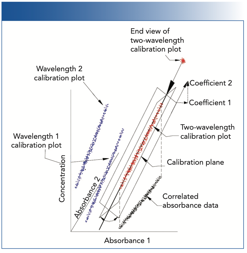
FIGURE 1: Illustration of the effect of intercorrelation of the calibration data on the determination of the calibration coefficients.

Figure 1 illustrates the difference between the situations where absorbance at one wavelength (or, strictly speaking, a small wavelength range represented by the central wavelength), and two (or more) distinct wavelengths with absorbances that are correlated are used to create a calibration model. Advanced discussions of calibration theory demonstrate analytically that intercorrelations between the variables of a regression analysis make the computed regression coefficients for those variables unstable, because of the increased sensitivity of the computed calibration coefficients to small changes in the data as the correlation of the absorbances at those wavelengths increases (5); in Figure 1, we present that situation graphically.
Figure 1 illustrates what happens when two correlated variables are both used in an attempt to “improve” the calibration. Because there are two independent variables (the absorbances at the two wavelengths), including the variable representing the concentrations, the data exist in a 3D space. Furthermore, the data are contained within a cylindrical region of that space. A calibration model, in this situation, is comprised of a plane representing the cylindrical shape of the data, rather than a line. This plane represents the least-square fit to the data. However, since the noise of the absorbances at the two wavelengths are random and of approximately equal magnitude, the exact position of the plane is very rotationally unstable, and subject to the influences of these very small fluctuations of the noise. The upper-right-hand corner of Figure 1 is a vector diagram (somewhat stylized, to be sure) showing how the projection of an extension of the plane against lines parallel to the axes of the space define the values of the two coefficients of the calibration. If the plane were to rotate around the axis shown, to a different position, then the projections would change in length, representing changes in the values of the calibration coefficients that we observed.
Figure 1 shows a representation of a two-wavelength calibration, and is one for which we can draw a diagram, which compresses a three-dimensional situation into the two dimensions of the figure. For a calibration using more than two wavelengths, an analogous figure would be required to represent four or more dimensions, which is beyond our capability to draw, and also beyond most people’s capability to visualize (including ours). However, the mathematics assures us that the same phenomena will create the instability we see in the two-wavelength, 3D case, in those higher-dimensional situations as well.
Therefore, we can explain the cause of what we observed as an apparent inability to reproduce a calibration model when using MLR technology, even though any calibration model resulting from a different orientation of the calibration plane would, in practice, perform equally well. However, this understanding does not provide us with a tool to correct the situation, or even give us a means to select, from all the possible orientations of the calibration plane, the one orientation, with its corresponding calibration coefficients that would allow other scientists to reproduce that exact model. Thus, as we discussed above in our introductory comments to this column, data transforms and modifications to the basic MLR algorithm were applied to address this issue and other problems that arose.
We will begin our examination of alternate calibration methodologies in the next column on this topic.
References
(1) J. Workman and H. Mark, Spectroscopy 32(10), 18–25 (2017).
(2) J. Workman and H. Mark, Spectroscopy 33(6), 22–26 (2018).
(3) H. Mark and J. Workman, Chemometrics in Spectroscopy (Elsevier, Amsterdam, The Netherlands, 2nd ed., 2018).
(4) H. Mark, Principles and Practice of Spectroscopic Calibration (John Wiley & Sons, New York, NY, 1991).
(5) N. Draper and H. Smith, Applied Regression Analysis (John Wiley & Sons; New York, NY, 3rd ed., 1998).
Jerome Workman, Jr. serves on the Editorial Advisory Board of Spectroscopy and is the Senior Technical Editor for LCGC and Spectroscopy. He is also a Certified Core Adjunct Professor at U.S. National University in La Jolla, California. He was formerly the Executive Vice President of Research and Engineering for Unity Scientific and Process Sensors Corporation.

Howard Mark serves on the Editorial Advisory Board of Spectroscopy, and runs a consulting service, Mark Electronics, in Suffern, New York. Direct correspondence to: SpectroscopyEdit@mmhgroup.com ●


NIR Spectroscopy Explored as Sustainable Approach to Detecting Bovine Mastitis
April 23rd 2025A new study published in Applied Food Research demonstrates that near-infrared spectroscopy (NIRS) can effectively detect subclinical bovine mastitis in milk, offering a fast, non-invasive method to guide targeted antibiotic treatment and support sustainable dairy practices.
Smarter Sensors, Cleaner Earth Using AI and IoT for Pollution Monitoring
April 22nd 2025A global research team has detailed how smart sensors, artificial intelligence (AI), machine learning, and Internet of Things (IoT) technologies are transforming the detection and management of environmental pollutants. Their comprehensive review highlights how spectroscopy and sensor networks are now key tools in real-time pollution tracking.
New AI Strategy for Mycotoxin Detection in Cereal Grains
April 21st 2025Researchers from Jiangsu University and Zhejiang University of Water Resources and Electric Power have developed a transfer learning approach that significantly enhances the accuracy and adaptability of NIR spectroscopy models for detecting mycotoxins in cereals.