Identifying Freshness of Shrimp Following Refrigeration Using Near-Infrared Hyperspectral Imaging

Shrimp tends to deteriorate during the refrigeration process. To monitor the freshness of shrimp during refrigeration, near-infrared (NIR) hyperspectral imaging was utilized to non-destructively identify the freshness of shrimp. In the process, three preprocessing methods (multivariate scatter correction [MSC], standard normal variate [SNV], and direct orthogonal signal correction [DOSC]) were employed to preprocess the full-wavelength spectral data, and three characteristic wavelength extraction algorithms (competitive adaptive reweighted sampling [CARS], and random forest [RF] simulated annealing [SA]) were used to extract the best-pre-processed data. Because extreme learning machine (ELM) and kernel extreme learning machine (KELM) are easily affected by parameters, ELM (based on teaching-learning-based optimization [TLBO]) and KELM (based on teaching-learning-based optimization [TLBO]) were proposed. In this study, four discriminant models (ELM, TLBO– ELM, KELM, and TLBO–KELM) were used for the full wavelength modeling analysis and the characteristic wavelength modeling analysis. In this work, the results of the final selected models are presented.

Shrimp is a food with high protein content (about 20%, which is higher than that of many fish, eggs, and milk [1,2]). Compared to fish, shrimp contains less essential amino acids and valine, making it a nutritionally balanced protein source. Shrimp is rich in glycine, which makes it taste sweet (3). Shrimp also has certain adjuvant therapeutic effects on skin ulcers, hand and foot convulsions, and neurasthenia; therefore, it potentially may have high medicinal value. Compared with poultry, shrimp has less fat content and almost no animal sugar as an energy source, making it highly nutritious (4). Shrimp is rich in taurine (which can lower the serum cholesterol level in the human body [5]), as well as potassium, iodine, magnesium, phosphorus, vitamin A, and vitamin B12. For these reasons, as well as many others, shrimp is very popular with consumers.

Shrimp are often processed into various seafood products (6); however, because of the action of microorganisms and their enzymes, they are vulnerable to quality damage during storage and transport (7). As a result, the short shelf life of shrimp severely affects their sale and distribution (8). Therefore, it is especially essential to identify the shelf life of shrimp in an accurate and timely matter (9,10).

The freshness of shrimp was traditionally identified using instruments for analysis and manual organoleptic evaluation (11–14). The instrument analysis method offers the inspector an approach to determine the chemical index of shrimp, such as pH value (15); unfortunately, this method has poor reliability and cannot be repeated. The artificial sensory evaluation necessitates the inspector to identify the odor and meat quality of the shrimp (16), so the method can be time-consuming and costly.

In recent years, many researchers have introduced hyperspectral imaging techniques with low cost and nondestructive testing characteristics to inspect a variety of products. Thus, it is extensively utilized in the area of freshness detection of food (17–19). Yu and associates used hyperspectral imaging technology to estimate the total volatile basic nitrogen (TVB-N) content of white shrimp, and obtained high precision (20). Wu and coauthors proposed a new method utilizing the fusion of spectral and image information to finally discriminate the freshness of salmon (21). Yao and associates achieved three freshness levels for egg sample classification by using a hyperspectral image acquisition system (22). Zhu and coauthors utilized two hyperspectral imaging systems to achieve freshness identification of spinach under different temperatures and storage time conditions (23). The near-infrared (NIR) spectral range makes the rapid imaging of samples particularly convenient, and the chemical composition difference within each pixel is shown by high-contrast images (24). Hyperspectral imaging allows simultaneous acquisition of distinct spectra and image information for every pixel on the surface of an object (25). The hyperspectral imaging (NIR band), which combines the above two advantages, is a good development prospect for the quality detection of aquatic products (26).

According to this investigation, it is feasible to utilize hyperspectral imaging to accurately identify refrigerated storage days for shrimp. The detail objectives of this study are as follows: (a) analyzing the peak distribution of the full spectral curves and the standard deviation of the average spectral curves for different refrigerated storage days of shrimp; (b) determining the best data preprocessing method to optimize the accuracy of full wavelength modeling; (c) extracting the characteristic wavelengths of the best preprocessed hyperspectral data using diverse algorithms; (d) using teaching-learning based optimization (TLBO) to optimize the parameters of the extreme learning machine (ELM) and kernel extreme learning machine (KELM) discriminant models; (e) modeling of characteristic wavelengths by using discriminant models to obtain the best-combined model for identifying refrigerated storage days for shrimp; and (f) visualizing classification results to provide more intuitive prediction results.

Materials and Methods

Sample Acquisition

The experimental samples were 420 white shrimp with an average weight of about 15 g. All the shrimp were placed individually in sterile bags, and then transported in foam incubators with fresh crushed ice by special vehicles to the laboratory. The preparation of samples was performed in the laboratory, where the shrimp were individually removed from the incubator, their heads and tails were removed, and what remained was washed in ice water. Then all samples were placed in a 4 ^oC incubator for different storage times (1d, 2d, 3d, 4d, 5d, 6d, and 7d). A total of 60 samples were labeled for each storage time (1–7 days), and we tested 60 samples/day for 7 d.

Hyperspectral Imaging System

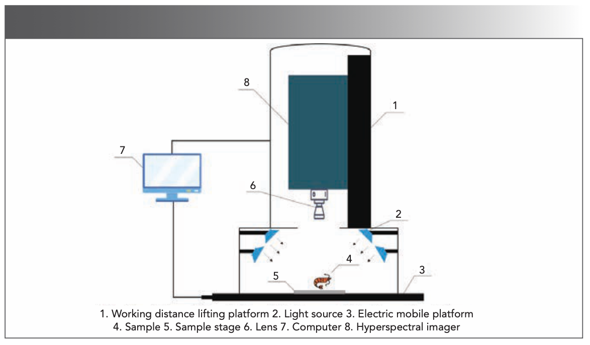
The hyperspectral imaging system is the “Gaia Sorter” near-infrared high spectrometer. As shown in Figure 1, the working mechanism of the “Gaia Sorter” near-infrared high spectrometer works as follows: A uniform light source illuminates a sample placed on an electronically controlled mobile platform, and the emitted light of the sample is captured by a spectral camera through the lens to obtain one-dimensional (1D) images and spectral information. With the continuous movement of the sample, it is possible to obtain continuous 1D images and realtime spectral information, and eventually a three-dimensional (3D) data cube containing image information and spectral information (27).

FIGURE 1: “Gaia Sorter” NIR high spectrometer main structure.

Hyperspectral Image Acquisition and Correction

Prior to using the NIR spectrometer, the light source was adjusted for maximum brightness. The electronically controlled mobile platform was stabilized (the standard whiteboard had been removed), and all electrical cables were connected. The original hyperspectral images of white shrimps were collected in groups of 4 samples, and 15 original hyperspectral images were collected per day for a total of 105 original hyperspectral images collected over the 7 days. To minimize the impact of the dark current of the CCD camera and the uneven intensity distribution of the light sources with different wavelengths, the original hyperspectral image required reflection correction (28). The correction formula is:

where C represents the corrected hyperspectral image, R represents the original image, B represents the all-black reference calibration image, and W represents the all-white reference calibration image.

Data Analysis

Spectral Data Extraction and Preprocessing

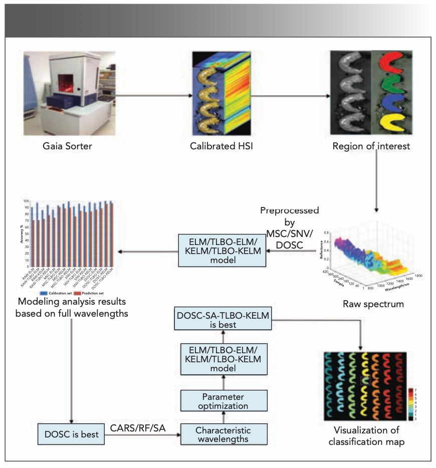
Because the original hyperspectral data is a hypercuube, a series of processes was required to finally obtain the spectral data (29). The process of spectral data extraction is shown in Figure 2. The specific steps are as follows: (a) opening the hyperspectral image corrected for reflectivity in ENVI 5.3 (ITT Visual Information Solutions); (b) selecting the entire area of each white shrimp as the region of interest (ROI); and (c) calculating the average reflectance for each wavelength of all pixels in the ROI, using them as spectral values of the sample; and then using Matlab2019a (The Math Works) to read the data, and to organize and add sample labels.

FIGURE 2: Main steps in the study (indicated by arrows).

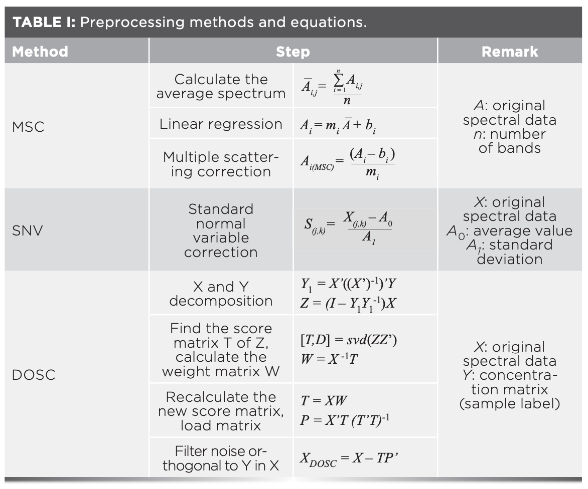
Because various noise sources are introduced in the original hyperspectral data acquisition process, it is necessary to preprocess the original spectral data. In this study, three spectral preprocessing methods (MSC, SNV, and DOSC) were respectively employed to preprocess the original spectral data. Table I shows the detailed steps and corresponding equations for the three preprocessing methods used.

Characteristic Wavelength Extraction

The highly redundant character of hyperspectral data will affect the robustness of subsequent models (30). However, this can be improved by using appropriate methods to extract the characteristic wavelengths. Competitive adaptive reweighted sampling (CARS), random frog (RF), and simulated annealing (SA) were used to extract characteristic wavelengths.

CARS is a variable selection method proposed in imitation of Darwin’s evolution theory of “natural selection.” First, a large number of samples are deleted based on Monte Carlo (MC) sampling. Second, the selection is made from the remaining wavelength variables by adaptive reweighted sampling (ARS) combined with PLSR. CARS can serve the purpose of efficiently finding the optimal combination of variables by selecting variables with large absolute regression coefficients in multiple Monte Carlo operations (31).

RF is a characteristic selection algorithm that jumps different models in model space, and does not require an a priori distribution (32). Its core idea is to construct an initial set of variables and a subset of candidate variables, and then calculate the probability of selecting an acceptable set of candidate variables; the higher the probability of selection, the more important the variables are to the model.

SA is a general random search algorithm, which is extended from the local search algorithm (33), simulating the principle of physical annealing of solids. The variables are put in an unordered state by initialization, then the new solution is calculated. The acceptance probability is then computed by using the evaluation function, and the current solution is output as the optimal solution when multiple successive new solutions are not accepted.

Optimization Method

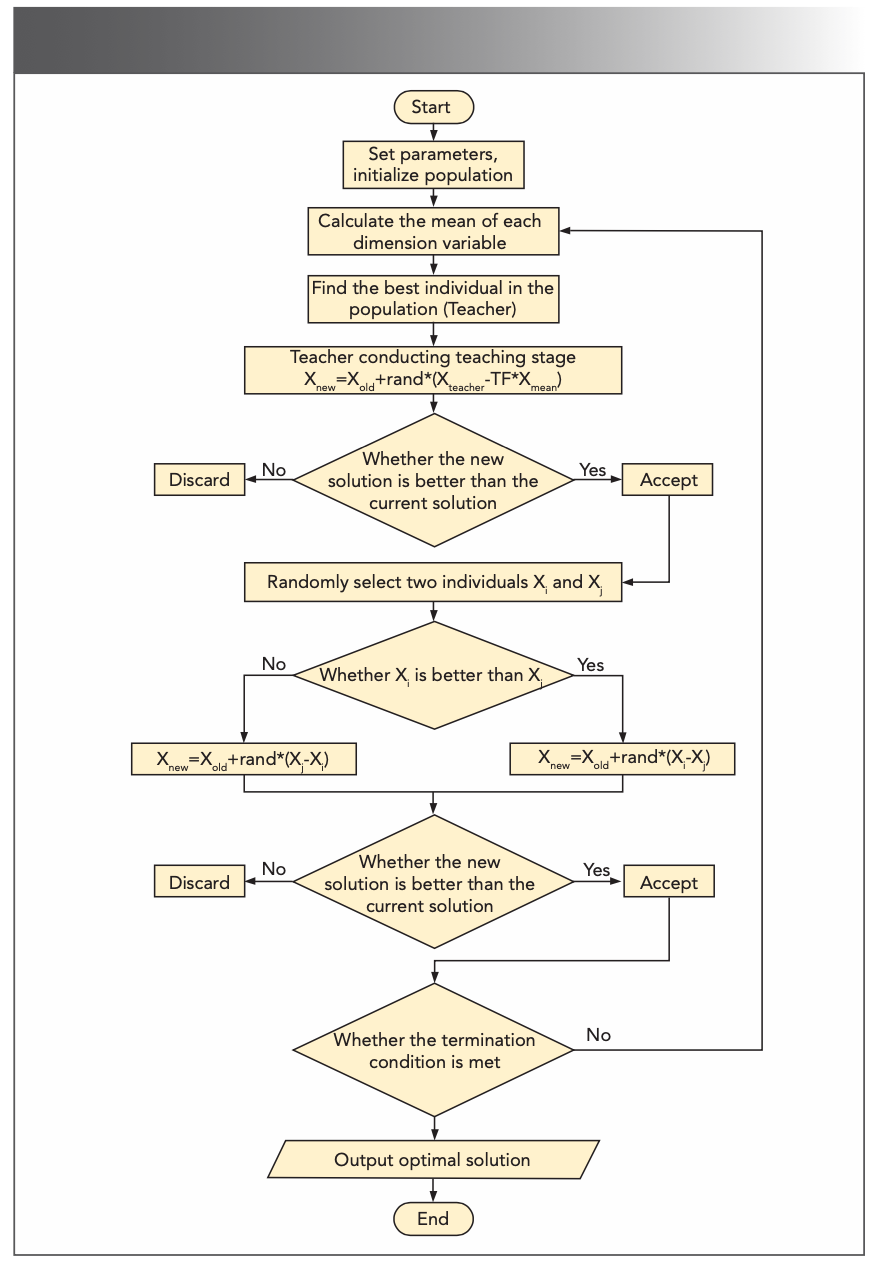
Rao and associates proposed TLBO in 2011 (34), which is a heuristic algorithm that simulates the teaching process. The flowchart of the algorithm is shown in Figure 3. In the “teaching” stage, teachers pass on their knowledge to students so as to narrow the knowledge gap between them. In the “learning” phase, a randomly selected object X_i is chosen in the class and adjusted by evaluating the differences between object X_i and student X_j. After each stage is completed, the population is updated by comparing it with the previous learning stage.

FIGURE 3: The flowchart of TLBO algorithm.

Discriminant Model

Extreme Learning Machine

ELM (or “over-limit learning machine”) is a type of machine learning system or method based on a feed-forward neural network (FNN), which is used to solve supervised learning and unsupervised learning problems (35). ELM is an improvement to FNN and its backpropagation (BP) algorithm. The ELM will randomly generate the connection weights between the input and hidden layers and the thresholds of the neurons in the hidden layer. ELM will not need to be adjusted during training; only the number of neurons in the hidden layer needs to be set to obtain the only optimal solution. Therefore, ELM improves the learning speed of the forward neural network so that the local minimum value or overfitting can be avoided.

Kernel Extreme Learning Machine

KELM is a new machine learning method formed by introducing kernel functions in ELM (36). The KELM does not need to set the number of nodes in the hidden layer of the network, but represents the non-linear feature mapping of the unknown hidden layer by the kernel function, and calculates the output weights of the network by the regularized least-squares algorithm. In this study, the radial basis function (RBF) kernel function is used, and its kernel parameter is represented by σ. Also, the parameter C was introduced to represent the regularization coefficient and to measure the output weights and training error.

Performance Evaluation

The reliability and accuracy of the performance of the prediction model are evaluated by the correct classification rate (CCR). The calculation formula is:

In equation 2, C represents the number of correctly classified samples, CCR represents the correct classification rate, and S represents the total number of samples.

Results and Discussion

Original Spectral Analysis

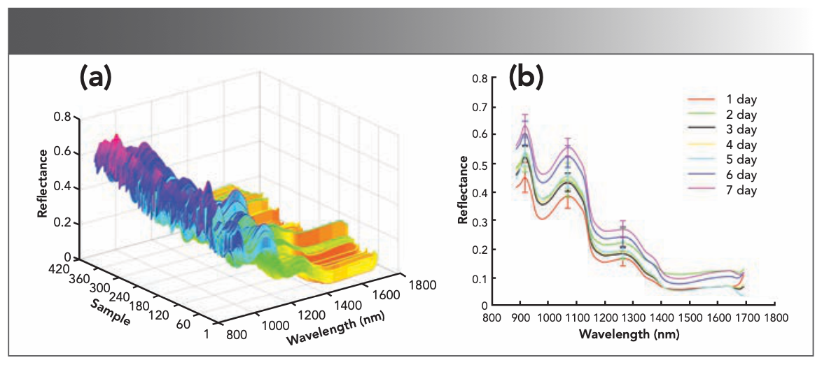
Figure 4a shows the original spectral curve. As can be seen from the graph, the largest reflectance is not larger than 0.8. The absorption peaks bands at 914.6 nm and 1259.0 nm correspond to the second overtone stretch of C-H. The 1064.8 nm absorption peak band corresponds to the second overtone stretch of N-H. Figure 4b shows the average spectral curves with their standard deviation of white shrimp on different refrigeration days. It can be seen that the sample dispersion degree is smaller under the same refrigeration time and the data is accurate. Also, the spectral curves of samples with different days of refrigeration are comparable, and it is difficult to distinguish in some bands. In the 1200–1300 nm band, the reflectivity progressively increases as the number of days of refrigeration increases.

FIGURE 4: (a) Original spectral curve, and (b) average spectral curves with their standard deviation of white shrimp on different refrigeration days.

Modeling Analysis Based on Full Wavelengths

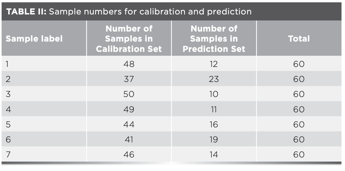
Before data analysis, the samples were divided into a calibration set and a prediction set. Sample set partitioning based on be x-y distances (SPXY) was developed based on the Euclidean distance method, and can enable efficient quantitative modeling of spectral analysis (37). This study used the SPXY method to divide the sample set in the ratio of 3:1. Table II shows the specific division of the sample calibration set and prediction set for different refrigeration days.

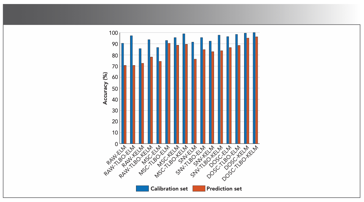
To select the optimal preprocessing method, the original spectral data, and the spectral data preprocessed by MSC, SNV, and DOSC were input into four discriminant models for comparison. Figure 5 shows the results of the full-wavelength modeling analysis of the above-preprocessing methods combining different discriminant models, in which RAW means the raw spectral data. It can be visualized that the spectral data processed by DOSC attained the highest modeling accuracy. The result comes from the difference between the sample itself and other factors. Before establishing the analysis model, DOSC is used to orthogonalize the spectral matrix and the label matrix to filter out information in the spectral matrix which is not related to the label matrix, so as to improve the accuracy of model classification (38).

FIGURE 5: Modeling analysis results based on full wavelengths.

Characteristic Wavelength Extraction Based on CARS, RF, and SA

To achieve the compression of the feature space dimension (that is, to obtain a set of data with a low probability of classification error), characteristic extraction is performed on the original data. In this study, CARS, RF, and SA were utilized to extract characteristic wavelengths from DOSC-processed spectral data (244 variables).

Figure 6a shows the results of running the CARS algorithm (set the number of Monte Carlo samples N = 100). The curve shows the decreasing number of variables selected as the number of samplings increases, and the rate of decline is from fast to slow. The curve (Figure 6b) shows a minimum RMSECV at the 64th sampling, showing that this sampling maximized the retention of useful information for identifying the number of refrigerated days. The curve (Figure 6c) shows the trend of the regression coefficients of wavelength variables during the optimization of wavelength variables, where “*” corresponds to the minimum RMSECV value. Finally, 11 characteristic wavelengths were selected using CARS, and Table III provides the interpretation of the relevant NIR spectral bands (39).

FIGURE 6: (a) Key variables selection results of competitive adaptive reweighted sampling (CARS). (b) Random frog (RF) variable screening results. (c) MSE of ANN in iterations of simulated annealing (SA). (d) The characteristic wavelengths correspond to the original spectral curve.

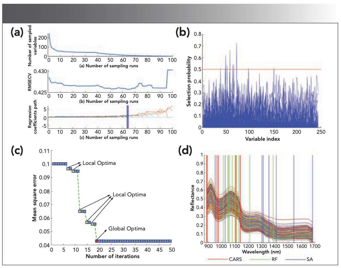
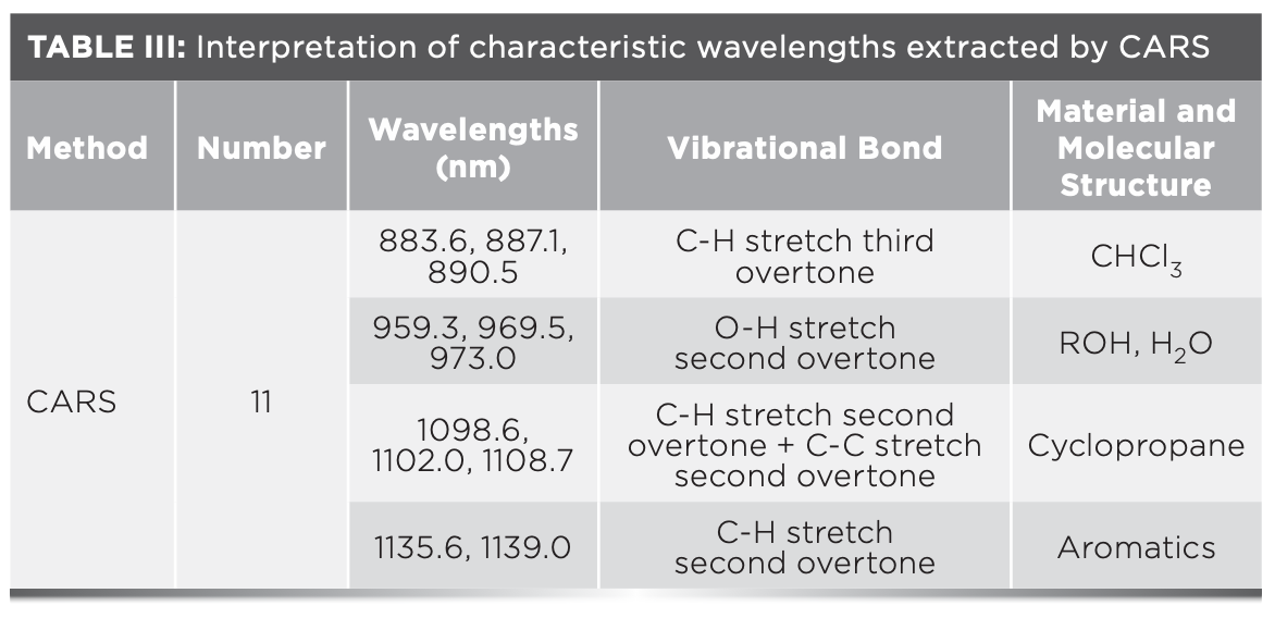
Figure 6b shows the probability of selection for each wavelength for which the RF algorithm was run 50 times and statistically averaged, revealing that only a small fraction of wavelengths exhibit a high selection probability, while most wavelengths exhibit a very low selection probability. This finding may represent a very small number of wavelengths, and thus provides a computational basis for demonstrating wavelength selection for the white shrimp refrigerated days discrimination. The threshold value was set at 0.5, and 10 characteristic wavelengths were finally selected. Table IV provides the interpretation of the relevant NIR spectral bands (39).

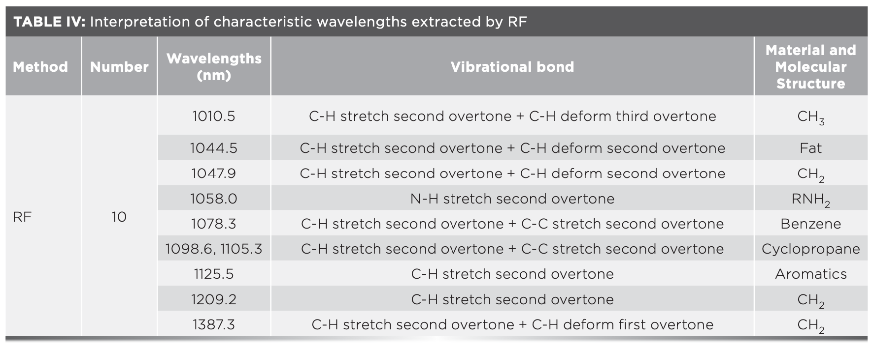
Figure 6c presents the convergence process of the MSE value during the SA iteration process. The evaluation function is the mean square error (MSE) of the artificial neural network (ANN) model. It can be seen from the figure that the 7th, 9th, 12th, 15th, and 17th iterations achieve the local optima respectively, the 19th iteration reaches the global optima, and the corresponding MSE value is 0.042 while outputting the optimal value. Finally, eight characteristic wavelengths were selected in the 19th iteration. Table V provides the interpretation of the relevant NIR spectral bands (39).

Figure 6d presents the distribution of characteristic wavelengths extracted by the three algorithms corresponding to the original spectral curves. It can be seen that the characteristic wavelengths extracted by CARS are mainly distributed near the first two absorption peaks, those extracted by RF are mainly distributed near the last two absorption peaks, and those extracted by SA are distributed at the three absorption peaks and the end of the spectral curve. The above results indicate that there is a lot of information near the absorption peak, and the correlation is strong. A high amount of C-H, O-H, and N-H are produced by the white shrimp with different refrigeration days during the protein and fat degradation process. Therefore, these characteristic wavelengths are strongly correlated with the number of refrigerated days for white shrimp.

Parameter Optimization

Before the modeling and analysis based on characteristic wavelengths, the non-optimized ELM discriminant model and the non-optimized KELM discriminant model adopt the method of random approximation to determine the model parameters, while the optimized ELM discriminant model and the optimized KELM discriminant model use TLBO to search for the optimal parameters.

One parameter of ELM is optimized by TLBO, and the parameter of ELM corresponds to the number of hidden layer neurons (L). The number of iterations is set to 30, the value range of L is within (0, 600), the initial population is 30, and the fitness function is the reciprocal of the correct classification rate of the prediction set (fitness [L] = 1/CCR). Figure 7a shows the convergence curve of the TLBO–ELM discriminant model. The data corresponding to the characteristic wavelengths extracted by CARS, RF, and SA was put into the TLBO-ELM discriminant model. During the parameter optimization process, as the iteration progresses, the extreme value of the fitness function value will be reached, thereby approaching the steady state. Under this condition, the optimal L is the output. The data corresponding to the characteristic wavelengths extracted by CARS are put into the TLBO–ELM discriminant model and the optimal output L is 37; the data corresponding to the characteristic wavelengths extracted by RF are put into the TLBO–ELM discriminant model and the optimal output L is 66; and the data corresponding to the characteristic wavelengths extracted by SA are put into the TLBO-ELM discriminant model (the optimal output L is 180).

FIGURE 7: (a) Convergence curve of TLBO-ELM discriminant model. (b) Convergence curve of TLBO-KELM discriminant model.

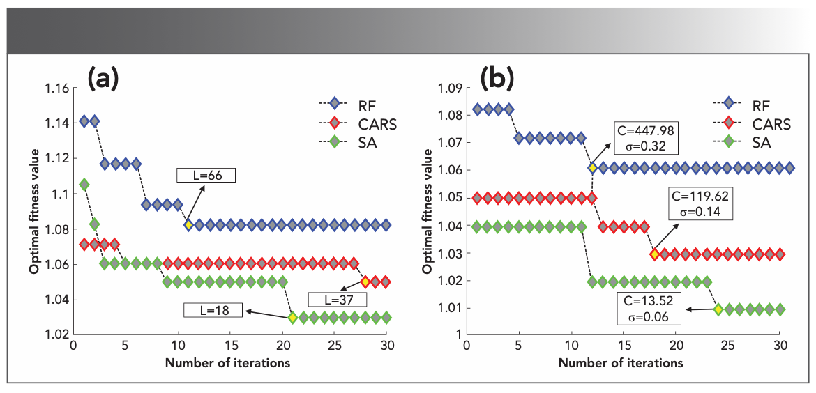
The two parameters of KELM, regularization coefficient (C), and kernel parameter (σ) are optimized by TLBO. The number of iterations is set to 30, the value range of C is within (0, 1000), the value range of σ is within (0, 2), the initial population is 60, and the fitness function is the reciprocal of the correct classification rate of the prediction set (fitness (C, σ) = 1/CCR). Figure 7b shows the convergence curve of the TLBO–KELM discriminant model. The data corresponding to the characteristic wavelengths extracted by CARS, RF, and SA was put into the TLBO–KELM discriminant model. During the parameter optimization process, as the iteration progresses, the extreme value of the fitness function value will be reached, thereby reaching the steady state. Under this condition, the output is optimal (C, σ). The data corresponding to the characteristic wavelengths extracted by CARS are put into the TLBO–KELM discriminant model and the output optimal (C, σ) is (119.62, 0.14); the data corresponding to the characteristic wavelengths extracted by RF are put into the TLBO–KELM discriminant model and the output optimal (C, σ) is (447.98, 0.32); the data corresponding to the characteristic wavelengths extracted by SA are put into the TLBO-KELM discriminant model and the output optimal (C, σ) is (13.52, 0.06).

Modeling Analysis Based on Characteristic Wavelength

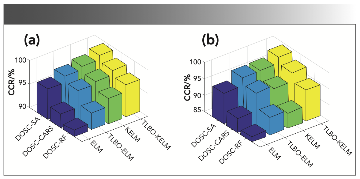
To further work out the optimal model combination, the data corresponding to the extracted characteristic wavelengths were entered into the ELM, TLBO-ELM, KELM, and TLBO-KELM discriminant models. Table VI shows the parameters of different models. Table VII shows the accuracy of the modeling analysis based on the characteristic wavelengths, and the overall classification results are satisfactory; all accuracy is exceeding 85%, indicating the validity of the selected characteristic wavelengths. To gain explicit analysis results, Figure 8a shows a 3D histogram of CCR values of different model calibration sets, and Figure 8b shows a 3D histogram of CCR values of different model prediction sets. It can be seen from the analysis of the two figures that: (a) TLBO-ELM compared to ELM, and TLBO-KELM compared to KELM, both with improved accuracy, indicates the effectiveness of the parameter optimization algorithm TLBO. (b) Different characteristic extraction algorithms (CARS, RF, and SA) were combined with the same discriminant model, where the SA algorithm combined with the same discriminant model achieved the highest classification accuracy by exceeding 94%, indicating that SA maximizes the removal of redundant information of the full wavelength and retains useful information, so the accuracy of the model is improved while CARS and RF do not show this result. (c) Different discriminant models (ELM, TLBO-ELM, KELM, TLBO-KELM) were combined with the same characteristic extraction algorithm, where the TLBO-KELM algorithm combined with the same characteristic extraction algorithm had the highest classification accuracy, and all exceeded 94%, which indicates that by TLBO-KELM, the most effective classification of data is achieved. In summary, the DOSC-SA-TLBO-KELM model achieved the optimal classification accuracy (99.37% and 99.05% accuracy for the calibration and prediction sets, respectively), so the DOSC-SA-TLBO-KELM model is selected as the optimal classification model.

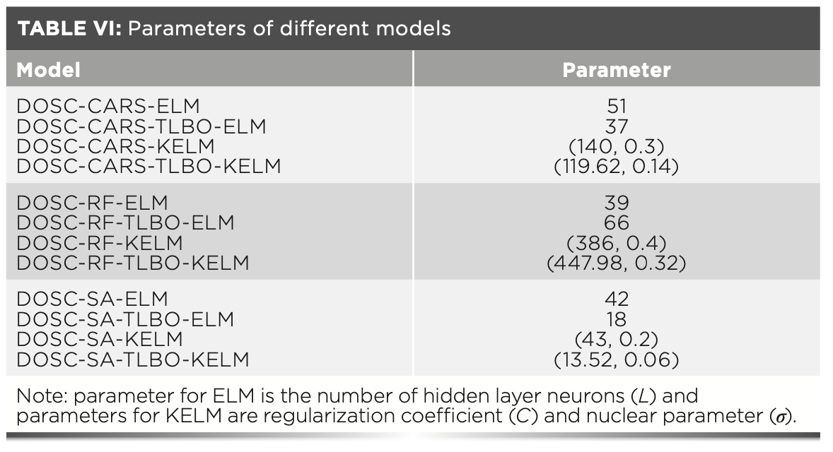
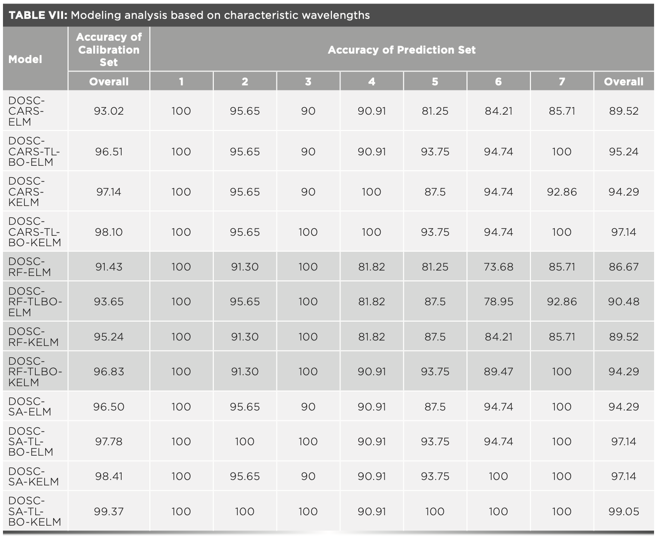
FIGURE 8: (a) CCR values of different model calibration sets. (b) CCR values of different model prediction sets.

In summary, the DOSC-SA-TLBO-KELM model achieved the optimal classification accuracy (99.37% and 99.05% accuracy for the calibration and prediction sets, respectively), so the DOSC-SA-TLBO-KELM model is selected as the optimal classification model.

Visualization of White Shrimp at Different Refrigerated Days

To interact with the data so as to clearly identify the number of refrigerated days for white shrimp, it is necessary to visualize the experimental results. Visualization is broadly divided into two approaches, object-wise and pixel-wise. The object-wise approach is based on mapping the entire sample average data attributes to corresponding pixels in the finite screen space. The pixel-wise approach is based on mapping each data attribute to a corresponding pixel in the finite screen space and reflecting the data distribution by arranging the pixels.

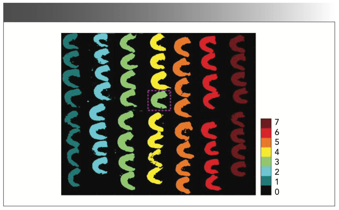
This study investigates the feasibility of classifying the number of refrigerated days of white shrimp. Therefore, this study uses the object-wise method for visualization. Bai and associates utilized hyperspectral imaging combined with chemometrics to identify maize seeds and used the object-wise method to visualize them (40). Each day, eight samples were randomly selected from the experimental samples; thus a total of 56 samples were produced. Figure 9 shows the classification results for the final visualization, in which each group of the white shrimps corresponds to the number on the right chromaticity bar, and the background value is 0. It can be seen that most classification results of white shrimp with different refrigeration days are right. Only one white shrimp on Day 4 was misclassified, and the overall classification accuracy was 97.92% (47/48). The visualization results indicate that the model developed in this study is reliable. Besides, the visual classification map facilitates rapid detection and timely removal of non-fresh white shrimps, thus ensuring their freshness.

FIGURE 9: Visualization of white shrimp at different refrigeration days.

Conclusions

In this study, near-infrared hyperspectral imaging was employed to discriminate white shrimp with different days of refrigeration and achieved good discrimination results. During the period, three spectral preprocessing methods (MSC, SNV, DOSC), three characteristic wavelength extraction algorithms (CARS, RF, SA), two traditional discriminant models (ELM and KELM), and two new discriminant models (TLBO–ELM and TLBO–KELM) were utilized. After multivariate data analysis, it was found that DOSC filtered out irrelevant information from the spectral matrix to improve the accuracy of model classification, SA could remove the full wavelength redundancy and retain useful information to the maximum extent possible, and TLBO–KELM could achieve the most effective data classification. Therefore, the DOSC–SA–TLBO–KELM model had the highest accuracy and was selected as the optimal model to identify the number of refrigerated days for white shrimp. (the accuracy of the calibration set and the prediction set peaked at 99.37% and 99.05% respectively). Finally, based on the object-wise method to visualize the classification results, which could judge the different refrigerated days of white shrimp intuitively. Therefore, this study can provide a theoretical basis for the development of a system to detect shrimp freshness online utilizing hyperspectral imaging technology.

Declaration of Competing Interest

All authors have no conflicts of interest.

Acknowledgment

This research was supported by Shandong Province Major Scientific and Technological Innovation Project (Project No.: 2019JZZY010703) and China’s National Key Research and Development Program (Project No.: 2017YFE0122100).

References

(1) Qiao, X.; Yang, L.; Gao, Q.; Yang, S.; Li, Z.; Xu, J.; Xue, C. Oxidation Evaluation of Free Astaxanthin and Astaxanthin Esters in Pacific White Shrimp During Iced Storage and Frozen Storage. J. Sci. Food Agric. 2019, 99 (5), 2226–2235. DOI: 10.1002/jsfa.9417

(2) Yu, L.; Jiang, Q.; Yu, D.; Xu, Y.; Gao, P.; Xia, W. Quality of Giant Freshwater Prawn (Macrobrachium rosenbergii) During the Storage at −18°C as Affected by Different Methods of Freezing. Int. J. Food Prop. 2018, 21 (1), 2100–2109. DOI: 10.1080/10942912.2018.1484760

(3) Yu, X.; Yu, X.; Wen, S.; Yang, J.; Wang, J. Using Deep Learning and Hyperspectral Imaging to Predict Total Viable Count (TVC) in Peeled Pacifc White Shrimp. J. Food Meas. Charact. 2019, 13 (3), 2082–2094. DOI: 10.1007/s11694-019-00129-0

(4) Dai, Q.; Cheng, J.; Sun, D.; Zhu, Z.; Pu, H. Prediction of Total Volatile Basic Nitrogen Contents Using Wavelet Features from Visible/Near-Infrared Hyperspectral Images of Prawn (Metapenaeus ensis). Food Chem. 2016, 197, 257–265. DOI: 10.1016/j.foodchem.2015.10.073

(5) Guo, J.; Duan, M.; Qiu, X.; Masagounder, K.; Davis, D.A. Characterization of Methionine Uptake and Clearance in the Hemolymph of Pacific White Shrimp Litopenaeus vannamei. Aquaculture 2020, 526, 735351. DOI: 10.1016/j.aquaculture.2020.735351

(6) Pan, C.; Chen, S.; Hao, S.; Yang, X. Effect of Low-Temperature Preservation on Quality Changes in Pacific White Shrimp, Litopenaeus vannamei: A Review. J. Sci. Food Agr. 2019, 99 (14), 6121–6128. DOI: 10.1002/jsfa.9905

(7) Zamora-Méndez, S.; Robles-Romo, A.; Marin-Peralta, E.; Arjona, O.; Apún-Molina, J. P.; Beltrán-Lugo, A. I.; Palacios, E.; Racotta, I. S. Postmortem Metabolic, Physicochemical, and Lipid Composition Changes in Litopenaeus vannamei in Response to Harvest Procedures. J. Aquat. Food Prod. T. 2017, 26 (7), 1093–1106 (2017). DOI: 10.1080/10498850.2017.1376236

(8) Le, N. T.; Doan, N. K.; Nguyen Ba, T.; Tran, T. V. T. Towards Improved Quality Benchmarking and Shelf Life Evaluation of Black Tiger Shrimp (Penaeus monodon). Food Chem. 2017, 235, 220–226. DOI: 10.1016/j.foodchem.2017.05.055

(9) Baptista, R. C.; Horita, C. N.; Sant’Ana, A. S. Natural Products with Preservative Properties for Enhancing the Microbiological Safety and Extending the Shelf-Life of Seafood: A Review. Food Res. Int. 2020, 127, 108762. DOI: 10.1016/j.foodres.2019.108762

(10) Olatunde, O. O.; Benjakul, S.; Yesilsu, A. F. Antimicrobial Compounds from Crustaceans and Their Applications for Extending Shelf-Life of Marine-Based Foods. Turk. J. Fish. Aquat. Sci. 2020, 20 (8), 629–646. DOI: 10.4194/1303-2712-v20_8_06

(11) Ghasemi-Varnamkhasti, M.; Goli, R.; Forina, M.; Mohtasebi, S. S.; Shafiee, S.; Naderi-Boldaji, M. Application of Image Analysis Combined with Computational Expert approaches for Shrimp Freshness Evaluation. Int. J. Food Prop. 2016, 19 (10), 2202–2222. DOI: 10.1080/10942912.2015.1118386

(12) Khodanazary, A. Freshness Assessment of Shrimp Metapenaeus affinis by Quality Index Method and Estimation of Its Shelf Life. Int. J. Food Prop. 2019, 22 (1), 309–319. DOI: 10.1080/10942912.2019.1580719

(13) Fang, Z.; Zhou, L.; Wang, Y.; Sun, L.; Gooneratne, R. Evaluation the Effect of Mycotoxins on Shrimp (Litopenaeus vannamei) Muscle and Their Limited Exposure Dose for Preserving the Shrimp Quality. J. Food Process. Pres. 2019, 43 (4), e13902. DOI: 10.1111/jfpp.13902

(14) Thimmappa, M. H.; Manjunatha Reddy, A.; Prabhu, R. M.; Elavarasan, K. Quality Changes in Deep-Sea Shrimp (Aristeus alcocki) During Ice Storage: Biochemical and Organoleptic Changes. Agric. Res. 2019, 8 (4), 497–504. DOI: 10.1007/s40003-019-00397-8

(15) Snellings, S. L.; Takenaka, N. E.; Kim Hayes, Y.; Miller, D. W. Rapid Colorimetric Method to Detect Indole in Shrimp with Gas Chromatography Mass Spectrometry Confirmation. J. Food Sci. 2003, 68 (4), 1548–1553. DOI: 10.1111/j.1365-2621.2003.tb09682.x

(16) Simoes, J. S.; Mársico, E. T.; De La Torre, C. A. L.; Mano, S. B.; Franco, R. M.; Santos, L. F. L. D.; Conte-Junior, C. A. Nutritional and Sensory Quality of the Freshwater Prawn Macrobrachium rosenbergii and the Influence of Packaging Permeability on its Shelf Life. J. Aquat. Food Prod. T. 2019, 28 (6), 703–714. DOI: 10.1080/10498850.2013.826769

(17) Feng, C.; Makino, Y.; Oshita, S.; García Martín, J. F. Hyperspectral Imaging and Multispectral Imaging as the Novel Techniques for Detecting Defects in Raw and Processed Meat Products: Current State-of-the-Art Research Advances. Food Control 2018, 84, 165–176. DOI: 10.1016/j.foodcont.2017.07.013

(18) Cheng, J.; Sun, D.; Zeng, X.; Liu, D. Recent Advances in Methods and Techniques for Freshness Quality Determination and Evaluation of Fish and Fish Fillets: A Review. Crit. Rev. Food Sci. 2015, 55 (7), 1012–1225. DOI: 10.1080/10408398.2013.769934

(19) Reis, M. M.; Van Beers, R.; Al-Sarayreh, M.; Shorten, P.; Yan, W. Q.; Saeys, W.; Klette, R.; Craigie, C. Chemometrics and Hyperspectral Imaging Applied to Assessment of Chemical, Textural and Structural Characteristics of Meat. Meat Sci. 2018, 144, 100–109. DOI: 10.1016/j.meatsci.2018.05.020

(20) Yu, X.; Wang, J.; Wen, S.; Yang, J.; Zhang, F. A Deep Learning Based Feature Extraction Method on Hyperspectral Images for Nondestructive Prediction of TVB-N Content in Pacific White Shrimp (Litopenaeus vannamei). Biosyst. Eng. 2019, 178, 244–255. DOI: 10.1016/j.biosystemseng.2018.11.018

(21) Wu, T.; Yang, L.; Zhou, J.; Lai, D. C.; Zhong, N. An Improved Nondestructive Measurement Method for Salmon Freshness Based on Spectral and Image Information Fusion. Comput. Electron. Agr. 2019, 158, 11–19. DOI: 10.1016/j.compag.2019.01.039

(22) Yao, K.; Sun, J.; Zhou, X.; Nirere, A.; Tian, Y.; Wu, X. Nondestructive Detection for Egg Freshness Grade Based on Hyperspectral Imaging Technology. J. Food Process Eng. 2020, e13422. DOI: 10.1111/jfpe.13422

(23) Zhu, S.; Feng, L.; Zhang, C.; Bao, Y.; He, Y. Identifying Freshness of Spinach Leaves Stored at Different Temperatures Using Hyperspectral Imaging. Foods 2019, 8 (9), 356. DOI: 10.3390/foods8090356

(24) Ndlovu, P. F.; Magwaza, L. S.; Tesfay, S. Z.; Mphahlele, R. R. Rapid Visible-Near Infrared (Vis-NIR) Spectroscopic Detection and Quantification of Unripe Banana Flour Adulteration with Wheat Flour. J. Food Sci. Technol. 2019, 56 (12), 5484–5491. DOI: 10.1007/s13197-019-04020-0

(25) Che, W.; Sun, L.; Zhang, Q.; Tan, W.; Ye, D.; Zhang, D.; Liu, Y. Pixel Based Bruise Region Extraction of Apple Using Vis-NIR Hyperspectral Imaging. Comput. Electron. Agr. 2018, 146, 12–21. DOI: 10.1016/j.compag.2018.01.013

(26) Toledo, M.; Gutiérrez, M. C.; Siles, J. A.; García-Olmo, J.; Martín, M. A. Chemometric Analysis and NIR Spectroscopy to Evaluate Odorous Impact During the Composting of Different Raw Materials. J. Clean. Prod. 2017, 167, 154–162. DOI: 10.1016/j.jclepro.2017.08.163

(27) Baek, I.; Kim, M.; Cho, B.; Mo, C.; Barnaby, J.; McClung, A.; Oh, M. Selection of Optimal Hyperspectral Wavebands for Detection of Discolored, Diseased Rice Seeds. Appl. Sci. 2019, 9 (5), 1027. DOI: 10.3390/app9051027

(28) Xiong, Z.; Sun, D.; Pu, H.; Xie, A.; Han, Z.; Luo, M. Non-Destructive Prediction of Thiobarbituricacid Reactive Substances (TBARS) Value for Freshness Evaluation of Chicken Meat Using Hyperspectral Imaging. Food Chem. 2015, 179, 175–181. DOI: 10.1016/j.foodchem.2015.01.116

(29) Wu, X.; Song, X.; Qiu, Z.; He, Y. Mapping of TBARS Distribution in Frozen–Thawed Pork Using NIR Hyperspectral Imaging. Meat Sci. 2016, 113, 92–96. DOI: 10.1016/j. meatsci.2015.11.008

(30) Sivertsen, A. H.; Kimiya, T.; Heia, K. Automatic Freshness Assessment of Cod (Gadus morhua) Fillets by Vis/Nir Spectroscopy. J. Food Eng. 2011, 103 (3), 317–323. DOI: 10.1016/j.jfoodeng.2010.10.030

(31) Hong, G.; Abd El-Hamid, H.T. Hyperspectral Imaging Using Multivariate Analysis for simulation and Prediction of Agricultural Crops in Ningxia, China. Comput. Electron. Agr. 2020, 172, 105355. DOI: 10.1016/j.compag.2020.105355

(32) Zhang, L.; Rao, Z.; Ji, H. NIR Hyperspectral Imaging Technology Combined with Multivariate Methods to Study the Residues of Different Concentrations of Omethoate on Wheat Grain Surface. Sensors 2019, 19 (14), 3147. DOI: 10.3390/s19143147

(33) Liu, D.; Sun, D.; Zeng, X. Recent Advances in Wavelength Selection Techniques for Hyperspectral Image Processing in the Food Industry. Food Bioprocess Tech. 2014, 7 (2), 307–323. DOI: 10.1007/s11947-013-1193-6

(34) Rao, R. V.; Savsani, V. J.; Vakharia, D. P. Teaching-Learning-Based Optimization: A Novel Method for Constrained Mechanical Design Optimization Problems. Comput. Aided Design 2011, 43 (3), 303–315 (2011). DOI: 10.1016/j.cad.2010.12.015

(35) Ye, R.; Chen, Y.; Guo, Y.; Duan, Q.; Li, D.; Liu, C. NIR Hyperspectral Imaging Technology Combined with Multivariate Methods to Identify Shrimp Freshness. Appl. Sci. 2020, 10 (16), 5498. DOI: 10.3390/app10165498

(36) Liang, J.; Yan, C.; Zhang, Y.; Zhang, T.; Zheng, X.; Li, H. Rapid Discrimination of Salvia Miltiorrhiza According to Their Geographical Regions by Laser Induced Breakdown Spectroscopy (LIBS) and Particle Swarm Optimization-Kernel Extreme Learning Machine (PSO-KELM). Chemometr. Intell. Lab. 2020, 197, 103930. DOI: 10.1016/j.chemolab.2020.103930

(37) Yuan, R.; Liu, G.; He, J.; Ma, C.; Cheng, L.; Fan, N.; Ban, J.; Li, Y.; Sun, Y. Determination of Metmyoglobin in Cooked Tan Mutton Using Vis/NIR Hyperspectral Imaging System. J. Food Sci. 2020, 85 (5), 1403–1410. DOI: 10.1111/1750-3841.15137

(38) Lin, M.; Wu, Y.; Rohani, S. Simultaneous Measurement of Solution Concentration and Slurry Density by Raman Spectroscopy with Artificial Neural Network. Cryst. Growth Des. 2020, 20 (3), 1752–1759. DOI: 10.1021/acs.cgd.9b01482

(39) Workman J.; Wryer, L. Practical Guide to Interpretive Near-Infrared Spectroscopy; CRC Press, Boca Raton, FL, 2007.

(40) Bai, X.; Zhang, C.; Xiao, Q.; He, Y.; Bao, Y. Application of Near-Infrared Hyperspectral Imaging to Identify a Variety of Silage Maize Seeds and Common Maize Seeds. RSC Adv. 2020, 10 (20), 11707-11715. DOI: 10.1039/C9RA11047J

Rongke Ye, Chunhong Liu, Daoliang Li, Yingyi Chen, Yuchen Guo, and Qingling Duan are with the College of Information and Electrical Engineering at China Agricultural University, in Beijing, China. Liu, Li, Chen, and Duan are also with the National Innovation Center for Digital Fishery at China Agricultural University, China. Direct correspondence to: sophia_liu@cau.edu.cn ●