Combining the WGAN and ResNeXt Networks to Achieve Data Augmentation and Classification of the FT-IR Spectra of Strawberries

It is essential to use deep learning algorithms for big data to implement a new generation of artificial intelligence. The effective use of deep learning methods depends largely on the number of samples. This work proposes a method combining the Wasserstein generative adversarial network (WGAN) with the specific deep learning model (ResNeXt) network to achieve data enhancement and classification of the Fourier transform infrared (FT-IR) spectra of strawberries. In this method, the data are first preprocessed using convolution, the FT-IR spectral data are augmented by WGAN, and the data are finally classified using the ResNeXt network. For the experimental investigation, 10 types of dimensionality-reduction algorithms combined with nine types of classification algorithms were used for comparing and arranging the 90 groups. The results obtained from these experiments prove that our method of using a combination of WGAN and ResNeXt is highly suitable for the classification of the IR spectra of strawberries and provides a data augmentation idea as a foundation for future research.

Fourier transform infrared (FT-IR) spectroscopy can be used to obtain biochemical fingerprints quickly and nondestructively, thereby providing a reliable molecular structure as well as composition information (1). These “spectral fingerprints” are unique to the substance being tested, which is conducive to the classification of the substance (2). At the same time, the continuous development of analytical techniques for different types of samples, high-throughput nondestructive analysis, and classification is ongoing (3). However, because the number of samples in the FT-IR spectral dataset is usually small, the research outputs obtained from spectral classification is limited (4).

Data augmentation, which is a well-known technique used for training neural networks to improve their robustness (5), is a particularly important strategy. Currently, it is used in many computer processing-driven fields (6), including image processing (7–9), speech processing (10,11), video processing (12), and several others. The core idea is to extend the newly generated samples from the original labeled data samples by simulating various expectations (13). In deep learning, the birth of the Wasserstein generative adversarial network (WGAN) has played an important role in data augmentation. The changes achieved by WGAN include solving the problems of training difficulty, fixing the instability of GAN, and preventing mode collapse. Furthermore, the smaller the loss function of GAN, the higher the quality of the corresponding generated data. The following are the key points in existing studies in the field of spectral data enhancement: (1) Each spectrum is shifted by a few wavenumbers randomly to the left or right; (2) a random noise is added, which is proportional to the magnitude at each wavenumber; and (3) for substances that have more than one spectrum, linear combinations of all spectra belonging to the same substance are taken as the augmented data. The coefficients in the linear combination are chosen at random (4). Random changes in the slope and random multiplications are added to the existing spectra to expand the dataset. The traditional methods prefer unsupervised data augmentation. However, in this work, we used supervised data augmentation. We found that WGAN is also suitable for data augmentation in the case of the IR spectrum. In addition, data augmentation significantly helped in data classification.

The classification of spectral data using convolutional neural networks (CNNs) has been studied to some extent (14,15), but the high-dimensionality and the smaller number of FT-IR spectra make it difficult to apply CNNs to them directly. At present, these networks are being used as classification models for analyzing spectral data (16). The ResNeXt network is a CNN with a special layout and restrictions, which is more suitable for data modeling (17). The traditional way to improve the accuracy of the model is to deepen or widen the network. However, as the number of hyperparameters increases, the difficulty of network design and the computational overhead will also increase. In contrast, the ResNeXt structure used in this work can improve the network accuracy without increasing the complexity of the parameters and using a small number of hyperparameters.

The common algorithm used in spectral classification research includes the classification algorithm or the dimensionality reduction algorithm combined with a classification algorithm. However, there are only a few types of these algorithms available. Therefore, in the exploratory experiments carried out in this work, we use the following algorithms: principal component analysis (PCA), t-distributed stochastic neighbor embedding (t-SNE), multidimensional scaling (MDS), local learning projection (LLP), locally linear embedding (LLE), Laplacian eigenmaps (LE), linear discriminant analysis (LDA), isometric feature mapping (ISOMAP), Autoender, independent component analysis (ICA) dimension reduction algorithms combined with the naïve Bayes classifier (NB), the k-nearest neighbor (KNN) classifier, logistic regression (LR), random forests (RFs), decision trees (DT), gradient boosting decision trees (GBDTs), support vector machines (SVMs), CNNs, and the long short-term memory (LSTM) classification algorithm. From the experimental investigations, we find that the combination of WGAN and ResNeXt, proposed in this work is highly efficient. During this experiment, preprocessing via convolution smoothing of 632 positive and 351 negative samples of the IR spectra of strawberries were performed. The IR spectral data were enhanced by WGAN to 3000 cases, and data classification was performed by the ResNeXt network. An overall accuracy of 99.72% was achieved, which takes into account 99.73% accuracy for precision0, 99.75% accuracy for recall0, 99.71% accuracy for precision1, and 99.69% accuracy for recall2. These percentages were obtained from the experiments.

Materials and Methods

Dataset Introduction

This work uses strawberry juice and non-strawberry juice FT-IR spectral datasets (from http://asu.ifr.ac.uk/example-datasets-for-download). The datasets were collected using the MonitIR FT-IR spectrometer at a nominal resolution of 8 cm^-1, and a total of 256 interferograms were added before carrying out their Fourier transform. A single-beam pure spectrum was compared with the background spectrum of water and then converted to absorbance units. The spectral range was truncated to 899‒1802 cm^-1 (235 data points) to remove the regions that are not needed for analysis. The absorption-mode spectrum acquisition interval under laboratory conditions was 3.86 nm.

Dataset Preprocessing

Because the environment of the entire system was constantly changing, the mea- sured spectra were often accompanied by a certain amount of inherent noise. The most commonly used denoising methods included moving average and Savitzky–Golay (S–G) convolution smoothing. The domain history is shown in Figure 1. We performed 5th-order S–G smoothing (5-point moving window and second-order polynomial) and 7th-order S–G smoothing (18,19). We chose the 5th-order S–G smoothing based on earlier studies (20).

FIGURE 1: FT-IR spectra for strawberries corresponding to the (a) average spectra, (b) spectra obtained by 5th-order Savitzky–Golay (S–G) smoothing, and (c) spectra obtained by 7th-order S–G smoothing.

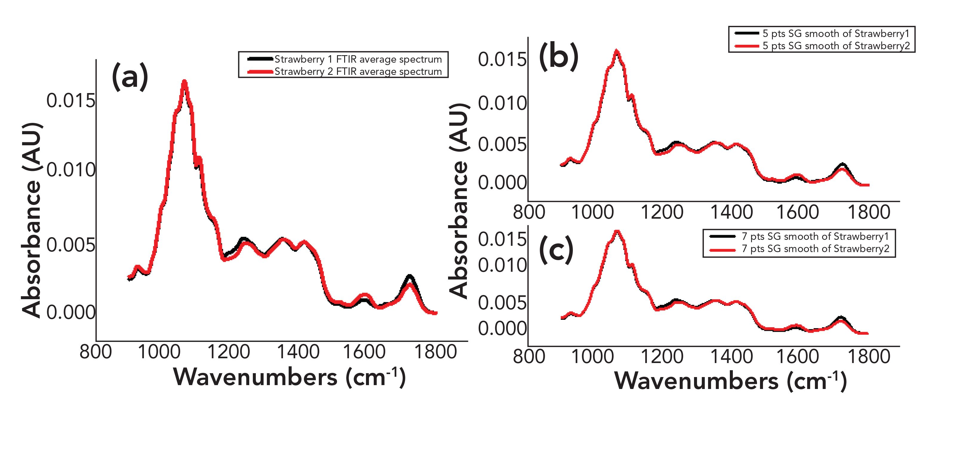
This approach is similar to the simple moving average idea, except that the S–G convolution method uses polynomials to perform polynomial least-squares fitting of the data in the window, eliminating simple data averaging, emphasizing the central point effect on the window and thereby reducing spectral noise. The following is the basic principle of S–G convolution smoothing in the spectrum.

Assuming that the original IR spectrum data is x, there are a total of m data points. The size of the sliding window is w, usually an odd number, which represents 2n + 1 consecutive points in the spectrum. Polynomial fitting of the spectral data is carried out in the window and the polynomial is determined as follows:

Among them j = -n, -n + 1,..., -1, 0, 1,... n−1, n represent the points 2n + 1 in the window, x_i+j represents the data points around the first data point, that is, the center point of the window, i = 1, 2, ..., m, a represent the polynomial coefficient, and k represents the highest degree of the fitting polynomial. It is not difficult to see that the formula expresses a total of 2n + 1 equations and requires k+1 coefficients to be solved. Therefore, it must be satisfied when S–G denoising is used; in other words, the selected window size should be larger than the polynomial coefficient. Furthermore, the formula can be expressed in a matrix form, as:

where X⁽ⁱ⁾ = (X_i+j⁽ⁱ⁾), A = (a_i), J is the Vandermonde matrix, namely:

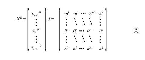
The least square method can be used to solve the problem, and the estimated value of A can be obtained as

By putting  into the formula, we can determine the estimated value of X⁽ⁱ⁾ as x_i.

The estimated value x⁽ⁱ⁾ in x_i⁽ⁱ⁾ is the result of S–G convolution smoothing under the sliding window. The reason why this method is called convolutional smoothing is not difficult to see from the formula, and the obtained value x_i⁽ⁱ⁾ is the j = 0 time value:

Let V = (J^TJ)^-1 J^T and assume:

Then the formula in matrix form can be given as:

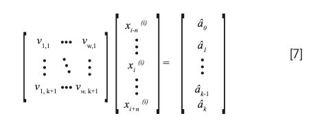
Then the combined formula can be obtained:

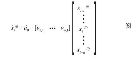
Then the formula can be written as convolution:

where v is the row vector [v_1,1 ... v_w,1] and the result is obtained after flipping along the center. It can be seen that the convolution coefficient of S–G convolution smoothing v does not depend on the spectral data, and only on the size of w, the sliding window and the highest degree of k polynomial fitting.

Model Introduction

WGAN

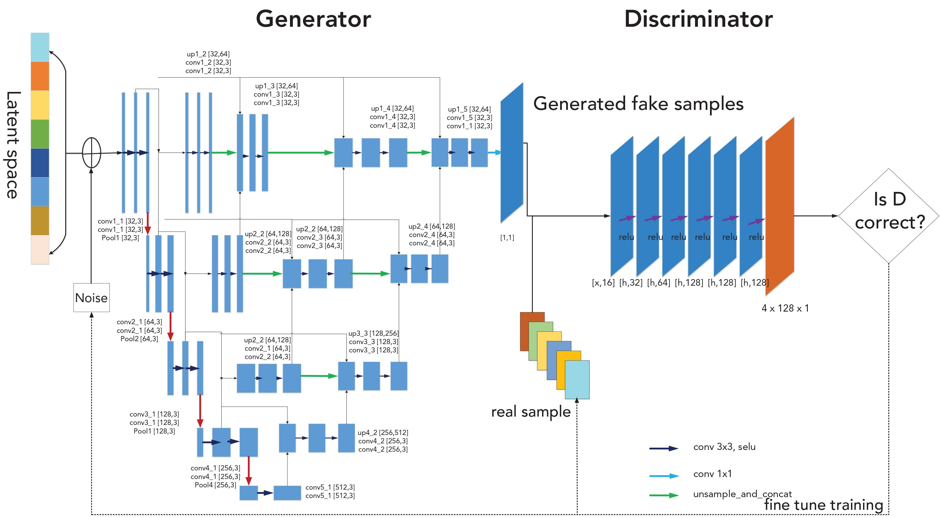
As shown in Figure 2, WGAN is composed of two parts: One is the generation mode, and the other is the discrimination mode. At first, in the original GAN version (21), the authors proposed two loss functions for the generation network, both of which have problems with gradients. The authors who developed WGAN elaborated on the problems of the training gradient in detail. They explained the reason for the model collapse from the perspective of distributed distance and proposed a new distance measurement method to ensure the smoothness of the gradient. This not only gets rid of the endless tuning process of balance discriminator and generative training, but it also enriches the diversity of the generative samples and avoids the same situation. It provides reliable numerical indicators to reveal the degree of training of the adversarial network (22).

FIGURE 2: The WGAN model.

The trends of the two spectra are very similar. To improve the degree of classification, we carried out data enhancement. To do this, the real spectrum of each sample is used as the input of the training data, and the generator model (G) generated 3000 random number sequences with the same output as the test data. The discriminator model (D) is used to distinguish the spectra. Regardless of the G model or the experimental spectrum, in the discriminator D, the labeling of the actual spectrum is different from the generated spectrum. In addition, the parameters of D are shared with G. In the original model and the generated spectrum, the G model is used as a training generator model. The real and the generated spectrum are labeled as the same. Finally, parameters are shared, and a new model spectrum is generated by the G model as the G output.

Generator Model

The network structure of the generator model is shown in the left half of Figure 2. It is divided into two processes—encoding and decoding. Its input is a noisy spectrum, and it generates an enhanced spectrum. Most of the noise comes from the random noise spectrum, which exhibits a nonlinear relationship with the clean spectrum. Thus, convolutional networks are used for extracting their relationship features, and the activation function, specifically the rectified linear unit (ReLU), is used for combining the relationship features to obtain an abstract spectral distribution feature. Based on the extracted features, spectral denoising can be performed. To further boost the enhancement effect, the generator model is designed as a fully convolutional U-Net structure without a fully connected layer. When the encoding–decoding part is not used, the network will skip the connection mode and will directly connect the encoding layer to the corresponding number of parameters and training time. At the same time, a pooling layer is added to select and sparse the extracted features to ensure optimal performance of the model. The number of filters in the coding layer are 32, 64, 128, 256, and 512, respectively. The convolution kernel has a size of three and a step size of two. During the encoding process, the data flows through the convolutional layer and the pooling layer. The encoding process is a mirror process of the encoding stage, that is, a deconvolution process, which is consistent with the encoding process parameter matching.

The U-Net structure was adopted by the generator in this work. The basic U-Net architecture is often used for medical image segmentation (23). However, using a basic model with low complexity cannot achieve the desired accuracy. To achieve a balance between the accuracy and model complexity (24), the U-Net connection was adjusted to extract complex features of the spectrum.

When inputting a set of information with an IR light intensity of 1 × 235, the data are first sent to the network. As seen from the network diagram, after the fifth convolution layer, upsampling for each subsequent layer is done. The operation is as follows: Because the model loses some information during the downsampling process, the relevant low-level features can be obtained during the upsampling process, so that the latter can get accurate features for the network. In addition, for lower resolution samples, one can get a larger number of characteristic parameters. In the IR spectrum image, U-Net does not need to understand the displacement characteristics of the FT-IR spectrum. For obtaining the prediction results of the network model, increasing the number of feature maps will not affect the experimental results.

Discriminator Model

The network structure for the discriminator model is shown in the right half of Figure 2. Its function is to distinguish the augmentation spectrum from the input spectrum and extract the probability of discrimination. Different types of noise have different distribution characteristics. Because of the differences between the enhanced spectrum obtained from the noisy spectrum and the original spectrum distribution, the original spectrum cannot be accurately simulated. The difference in the features is then extracted by a CNN as a basis for distinguishing between the original spectrum and the generated spectrum. The discriminator model is similar to the convolution design of the generator model. The number of filters is 16, 32, 64, 128, 128, 128, and 128. The size of the convolution kernel is three and the step size is two. Adding a batch of standardized layers on the network can reduce the impact of the initialization parameters on the training result and speed up the training. In this work, the leaky ReLU was used as the activation function.

Finally, the fully connected layer is added to output the discriminator result. In the discriminator model, the data first goes through the merged layer and then through the convolutional layer. The result is finally outputted through the fully connected layer.

ResNeXt

Figure 3 illustrates the The ResNeXt network, which is an improved version of the ResNet network (25). The ResNeXt structure can provide output with improved ac- curacy without increasing the complexity of the parameters and with a small number of hyperparameters. The visual geometry group (VGG) (26) stacking and the split- transform-merge feature of the inception module has strong scalability, which increases the accuracy while essentially not changing or reducing the complexity of the model. In the ResNeXt model, utilizing aggregated transformations have been proposed. The three-layer convolutional blocks of the original ResNet are replaced with blocks of the same topology that are stacked in parallel. The accuracy of the model is improved without significantly increasing the number of parameters. The structure is the same, and the hyperparameters are relatively reduced, which is convenient for model transformation.

FIGURE 3: The ResNeXt model.

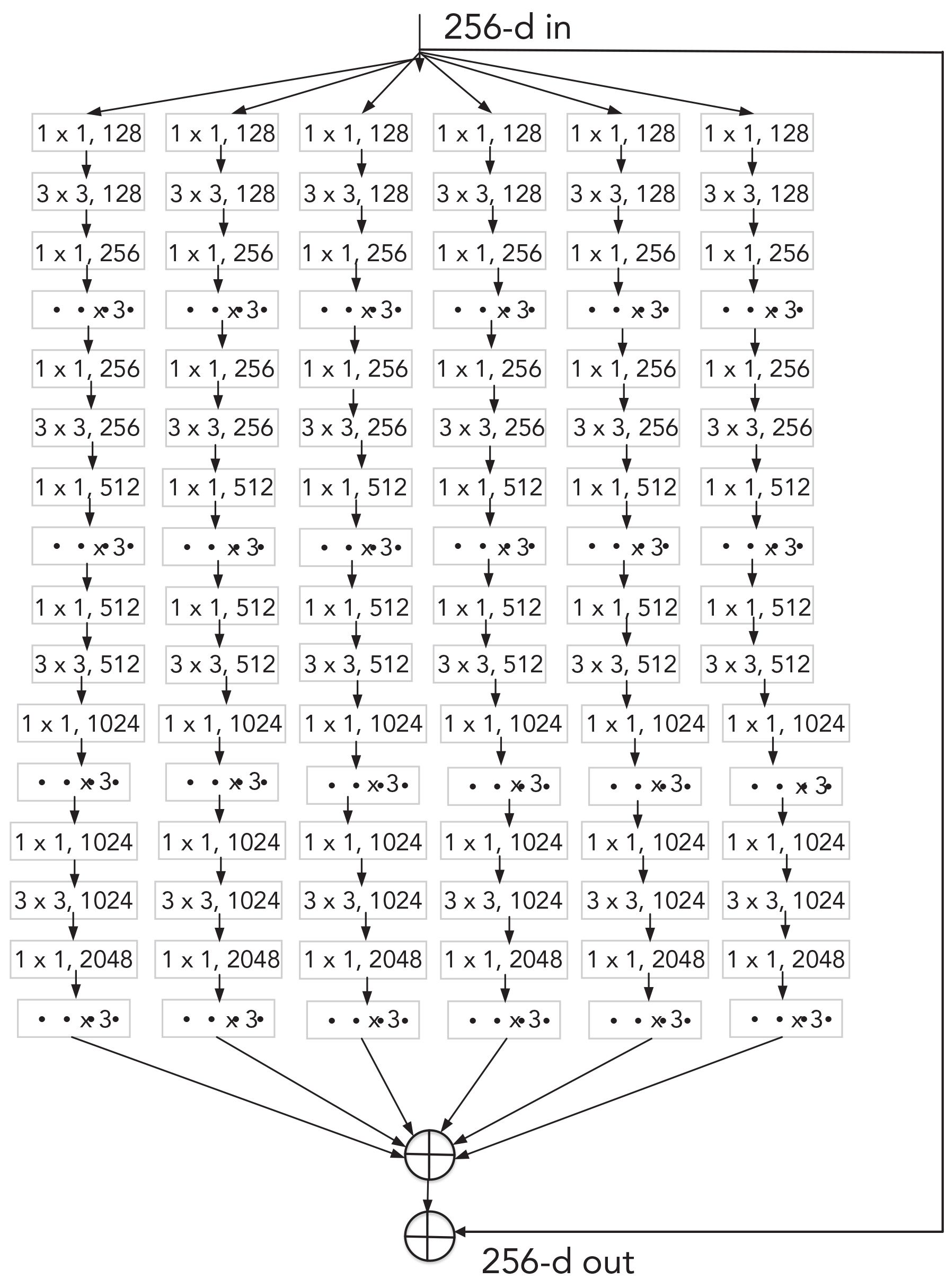
Within the ResNeXt framework, a strategy of deep separable convolution between ordinary convolution kernels has been proposed, in which packet convolution, which controls the number of packets (cardinality) to achieve a balance between the two strategies, is carried out. The idea of group convolution has been derived from the inception module. Unlike the inception module, which needs to manually design each branch, the topology of each branch of ResNeXt is the same. Combined with the residual network, the final ResNeXt is obtained. The structure of ResNeXt is very simple; however, a residual network of the same framework is obtained on ImageNet (27).

Compared to Inception 4, ResNeXt has fewer hyperparameters than those in Inception v4 (28). We applied ResNeXt to the IR spectrum classification and found that the effect is also applicable.

To improve the accuracy of the model, most of the existing deep learning methods usually deepen or widen the network, but as the number of hyperparameters increases, the difficulty and computational overhead involved in the network will also increase. The ResNeXt structure was first applied to the field of image classification and was found to be useful in improving the accuracy without increasing the complexity of the parameters.

The specific calculation formula of the ResNeXt structure is shown in formula 10, with x representing the input feature, T_i representing any function where it is a stack of three convolutional layers, and C representing the network input width.

Results and Discussion

Evaluation Criteria

In the experiments carried out in this work, the data are divided into a training set and a test set at a ratio of 4:1 using five-fold cross-validation. For performance evaluation, a confusion matrix has been used, which gives a numerical evaluation of the classification between paired categories. To effectively evaluate the performance, knowing the following definitions are integral:

• Classification accuracy: the ratio of the total number of samples classified correctly to the total number of samples.
• Precision: a measure of accuracy, representing the proportion of positive examples that are actually classified as positive examples.
• Recall: this indicates the proportion of all positive examples that are paired and measures the ability of the classifier to recognize positive examples.
• F1 score: it is a comprehensive consideration of precision and recall values.

Important Spectral Regions

The interpretation of the model is very important in the classification of chemical substances. Whether it is in the data enhancement or spectral classification, the main part of deep learning is the difference in the spectra. These differences contain the differences in the contents of the various chemical elements of the corresponding substances in different spectra. Based on the differences in the spectra of the two types of fruit juices studied in this work, the main regions of interest corresponding to the FT-IR shift are 899–956, 1057–1080, 1096–1116, 1122–1158, 1168–1263, 1298-1339, 1515–1619, and 1692–1762 cm^-1, of which the peaks in the regions 899–916 cm^–1 and 1057–1120 cm^–1 most probably correspond to ethanol. The peak around 880–1064 cm^–1 is a carboxyl group, and that around 1055 cm^–1 is related not only to alcohols but also to esters. The 1096–1116 cm^–1 interval is mainly affected by alcohol, 1168–1263 cm^–1 region has peaks because of the effect of ester, 1190–1350 cm^–1 corresponds to the phosphoryl group, 1575–1705 cm^–1 is the amide, 1692–1762 cm^–1 is mainly the absorption of water, and the peaks corresponding to lipids is 1708–1780 cm^-1. Some researchers have collected and analyzed volatiles from strawberries and found that the main components of the gas are esters, alcohols, furans, aldehydes, terpenoids, aromatic compounds, ketones, acids, and similar compounds (29–31). Ester is the main substance of strawberry volatilization. As esters are converted into fatty acids, the number of esters may decrease (32).

The range between 900–1200 cm^–1 deserves a special explanation. This region is also known as the “fingerprint area” of sugar and shows a significant difference between the juice groups (33). The main vibrational modes absorbing in this region are related with the C−O−C glycosidic linkage, the δCOH, and the vC−C.

Because it is difficult to assign a vibration mode corresponding to each individual frequency band, the frequency bands in this region collectively provide a complex pattern. The presence of fructooligosaccharides in the juice can be identified by the strong bands at 1134, 1034, and 935 cm^-1. A band at 1055 cm^-1 was observed in all groups due to sucrose. A typical sucrose band appears at 1054 cm^-1. A decrease in fructose peak indicates its hydrolysis and is consistent with the metabolism of yeast and mold. The band at 1037 cm^–1 is attributed to an increase in glucose, which is attributed to the hydrolysis of fructose at 986 cm^-1. Glucose, sucrose, and citric acid appear at 1029–1045, 1058–1061, and 1351–1378 cm^–1 (34). The vC vibration mode of the ester at 1724 cm^-1, exhibiting higher stability in all fiber-rich fruit juices, corresponds to the vCH vibration mode. Organic acids (fructose and galacturonic acid methyl ester) and organic acids at 1634 cm^–1 are embedded in water molecules in the juice base. The vibrational mode of vCH₂ produces an energy band of about 1400 cm^–1 (35).

Experimental Flowchart

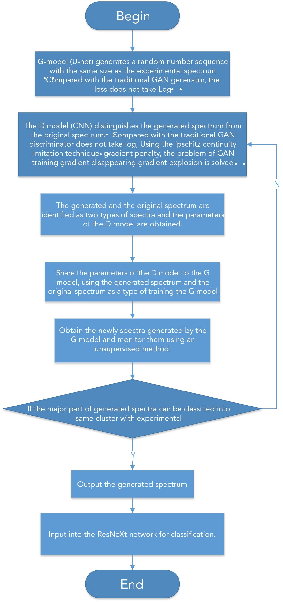
Figure 4 shows a flowchart of the experiment carried out in this work.

FIGURE 4: Experimental flowchart.

Training Process

The network training is done as per the flowchart shown in Figure 4. First, the noisy spectrum is used to train the generator model. Here, the noisy spectrum is encoded and decoded by the model to generate an enhanced spectrum and is then input into the discriminator model together with the noisy spectrum to generate an enhanced spectrum and is then combined with the noisy spectrum. The generated and the original spectra are simultaneously inputted into the discriminator model and compared. The network parameters are updated using the loss function defined by WGAN, and the generator model competes with the discriminator model. Over continuous iterations, the generated spectrum gradually approaches the original spectrum, thereby achieving spectral enhancement.

In this experiment, the generator model, G, directly processes the randomly generated curve signals, and the output is an enhanced spectral signal. The data first passes through the convolution operation and then enters the next layer of the network through the ReLU activation function. At the time of decoding, after entering the deconvolution block, the data passes through the ReLU activation function to enter the next layer of the network.

Figure 5 shows the optimization process of the generator model. The process is as follows: The weight parameters are adjusted according to the output of the discriminator model and the difference between the generated and the original spectrum. The input of the discriminator model D comes from two parts: one is the noisy light signal, and the other is the output of the model or the original spectral signal. After combining the data, a series of convolution operations is performed. The layer outputs the discrimination result.

FIGURE 5: Flowchart showing the optimization of the generator model.

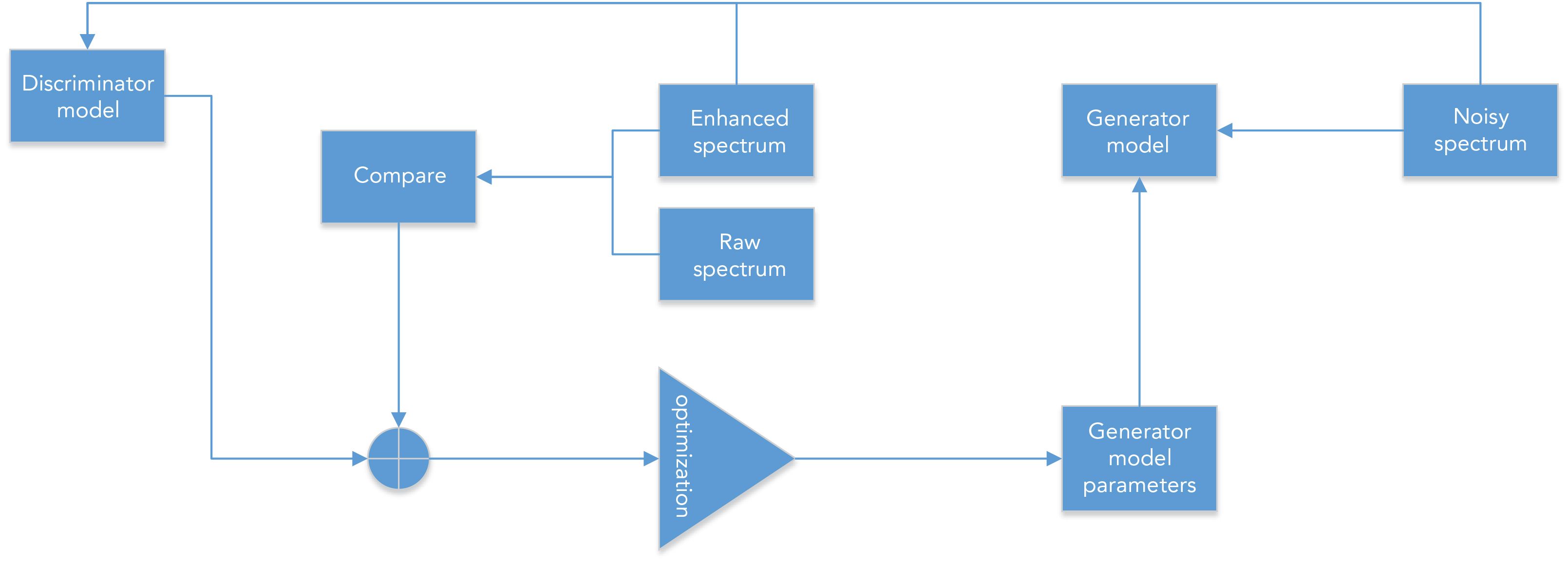
Figure 6 shows the decision-making optimization process of the discriminator model. The generator model generates an enhanced signal. The discriminator model then compares and classifies the noisy spectrum with the original spectrum and continuously adjusts the weight parameters during the iteration process.

FIGURE 6: Flowchart showing the decision-making discriminator model optimization process.

In this work, the use of spectral enhancement to generate an adversarial network has the following advantage: The network only uses backpropagation. The actual results show that WGAN can produce better spectral data. At the same time, during the training process, there is no need to manually extract spectral feature values, and it is not necessary to make inaccurate assumptions about the independence between the noise spectrum and the original spectrum. A well-searched network has generalization capabilities, which can enhance common noise.

Comparative Test

In the study of spectral classification, we can often see classification algorithms or reduction algorithms coupled with classification algorithms, and there are related studies that introduce data enhancement methods into spectral research (36,37). This article also introduces data enhanced algorithm.

In the first set of experiments, we introduce a combination of more traditional dimensionality reduction algorithms and classification algorithms. All the data in this set are used without enhancement.

All models use the Keras and Tensor-Flow libraries on the python platform, and the process is accelerated using the GPU.

Generally, a combination of a dimensionality reduction algorithms and classification algorithms is commonly used in experiments. We have performed 90 sets of comparative experiments, which are permutations and combinations of 10 sets of dimensionality reduction algorithms and nine sets of classification algorithms. They are PCA, t-SNE, MDS, LLP, LLE, LE, LDA, ISOMAP, Autoender, ICA dimensionality reduction algorithm combined with NB, KNN, LR, RF, DT, GBDT, SVM, CNN, and LSTM classification algorithm. The results thus obtained are shown in Figure 7.

FIGURE 7: Heat map of experimental results obtained using traditional methods.

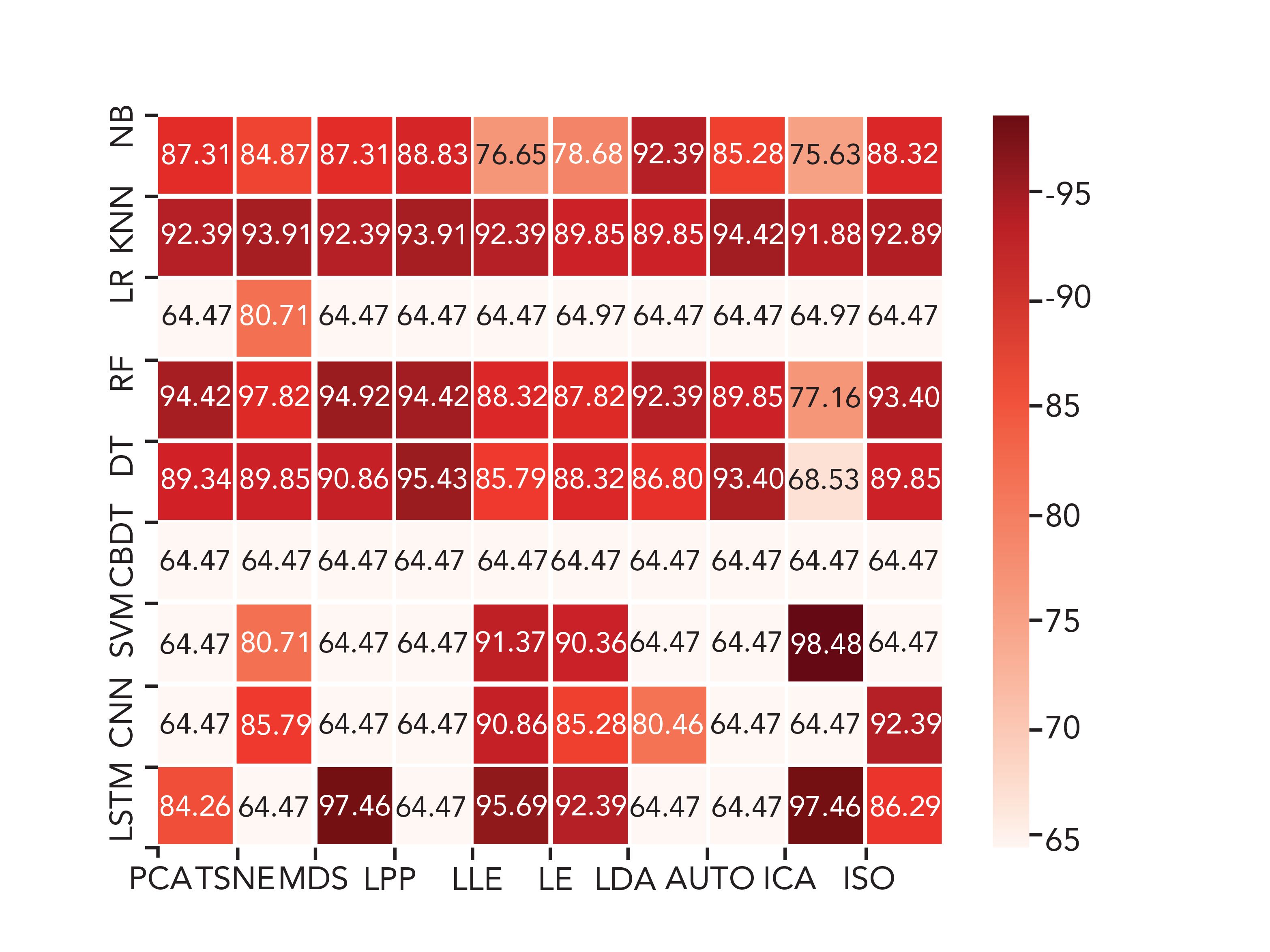
In the figure, the first seven are the behavioral machine learning algorithms, and the last two are the behavioral deep learning algorithms. From the results obtained, we can conclude that the algorithm with the best overall classification effect is KNN and the best overall dimensionality reduction algorithm is LLE, whereas the effect of CBDT on this dataset is relatively worse. On the basis of all the numerical values shown in Figure 7, the best combination algorithm is ICA-SVM. However, the effective use of machine learning and deep learning depends to a large extent on the number of samples. The small number of samples limits the effects of machine learning and deep learning. Therefore, in the second set of experiments, we use all the enhanced data at the same time, which are fed into the machine learning models and deep learning models.

In the past two years, deep learning has gained an increased interest in its use in IR spectroscopy studies. In our experiments, two representative deep learning networks, CNN and LSTM, were selected. CNN has been widely used in studies on multiple spectra.

Figure 8 shows the working of the CNN algorithm, which consists of a convolutional layer, a pooling layer, and a fully connected layer. The convolutional layer is composed of conv1D, dropout, and batch normalization. The pooling layer (shown in gray color) consists of a maximum pooling and a dropout layer. The fully connected layer is shown by the square piece in the figure. The flatten block flattens the data and sends it to the dense layer. The sigmoid activation function, namely, the Adam optimizer, is used.

FIGURE 8: Block diagram of the CNN model.

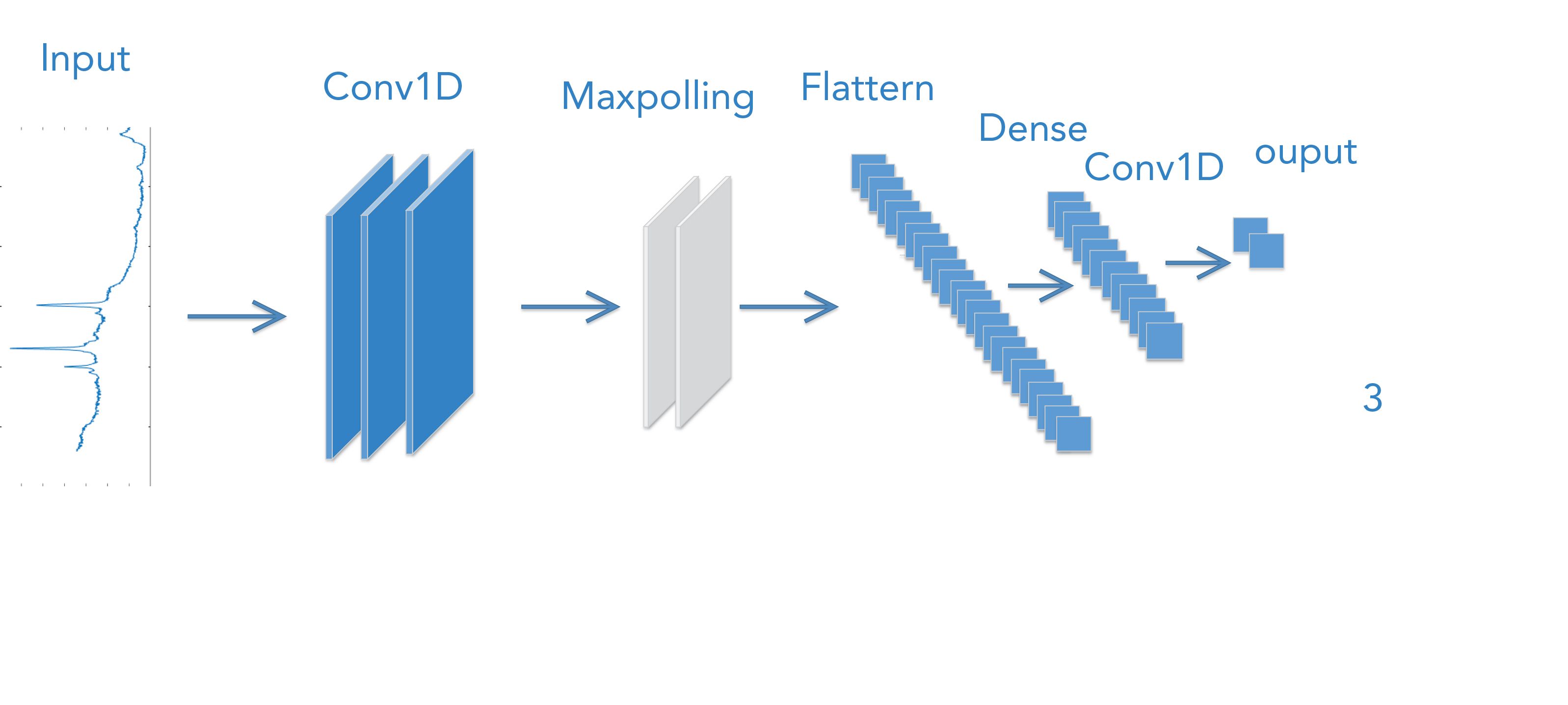
Figure 9 shows the block diagram of the LSTM algorithm, the second model used in this work. There are forget gates, input gates, and output gates in LSTM. A sigmoid layer called the input gate layer determines which spectral information needs to be updated; a tanh layer generates a vector, which is the alternative content to be updated. Next, the two parts are combined to perform an update of the state of the cell. A sigmoid layer is run to determine which part of the cell state will output. Next, the cell state is processed through the tanh to get a value between -1 and 1 and is then multiplied by the output of the sigmoid gate. In this way, only those parts that we require can be outputted.

FIGURE 9: Block diagram of the LSTM model.

To compare the experimental effects of traditional methods after enhancement, we introduced data enhancement on the basis of the first set of experiments and put all the enhanced data into the previous 90 sets of comparative experimental groups.

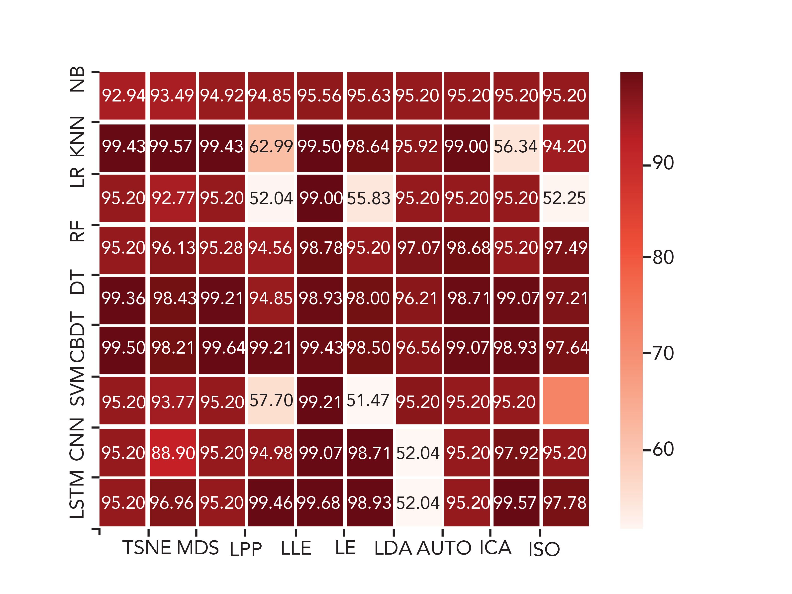
To verify the effect of data enhancement, we put all the enhanced data into all machine learning and deep learning and found that the classification effect of most algorithms has been significantly improved. Among them, NB, RF, DT, and CBDT algorithms attain more than 90% accuracy, and the best experimental accuracy of 99.68% was obtained for LLE-LSTM.

As shown in Figure 10, compared with the first set of experiments, irrespective of we employed machine learning or deep learning algorithms in the above experiments, the accuracy of the experiment is considerably improved after WGAN data is enhanced.

FIGURE 10: The heat map shows the experimental results obtained by the traditional method after applying WGAN.

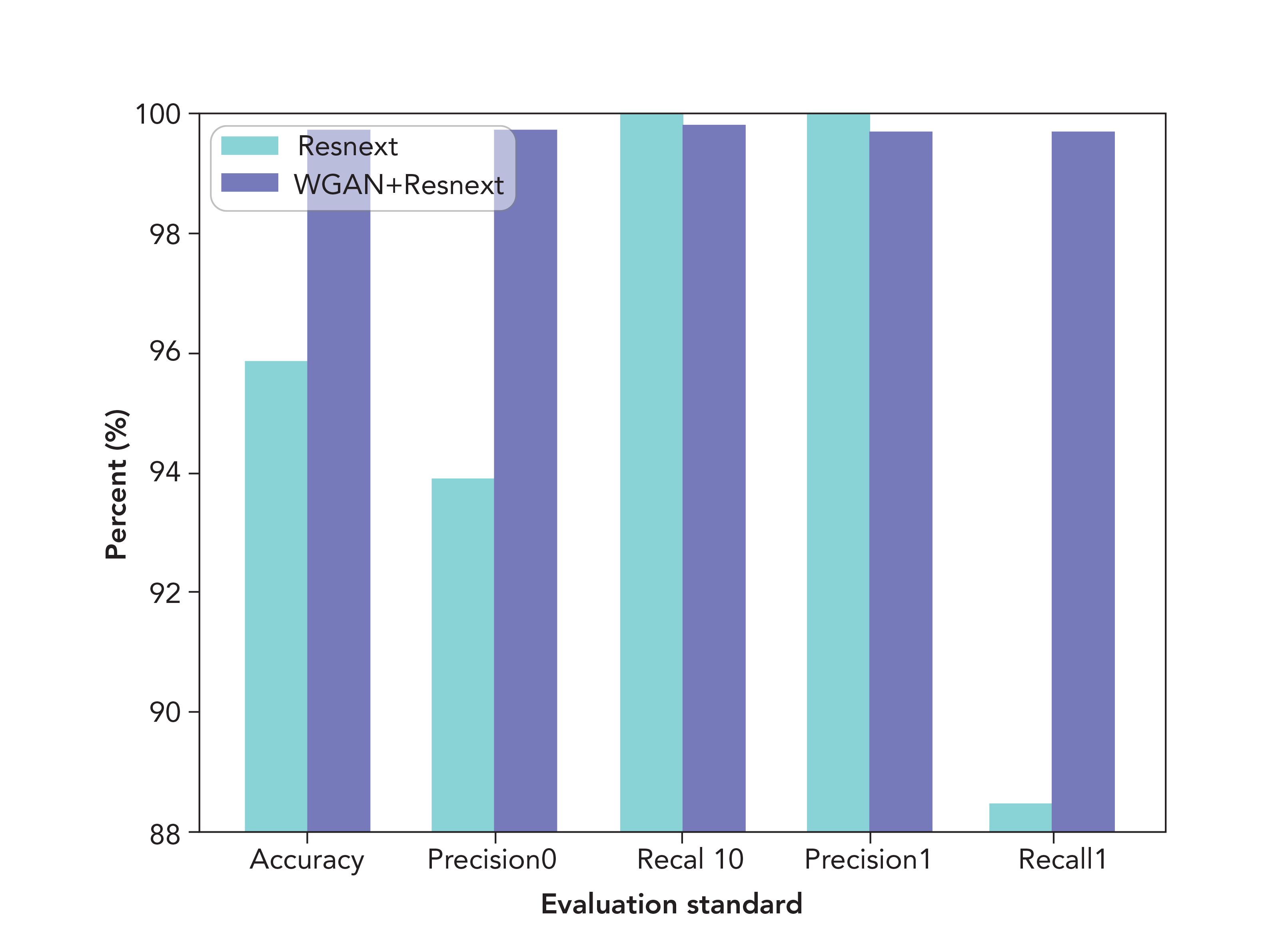
In the third set of experiments, we introduce the ResNeXt classification algorithm into the experiment. From the histograms shown in Figure 11, it can be clearly seen that the application of WGAN in combination with ResNeXt significantly improves the spectral data as compared to applying the ResNeXt network alone. An increase by 3.89% in accuracy, 5.85% in precision0, -0.25% in recall0, -0.29% in precision1, and 11.23% in recall1, is observed. In addition, it has the best performance compared to all previous experiments. The use of WGAN, in combination with LLE and LSTM, also improves the results by 0.04%.

FIGURE 11: Results obtained before and after the use of WGAN + ResNeXt.

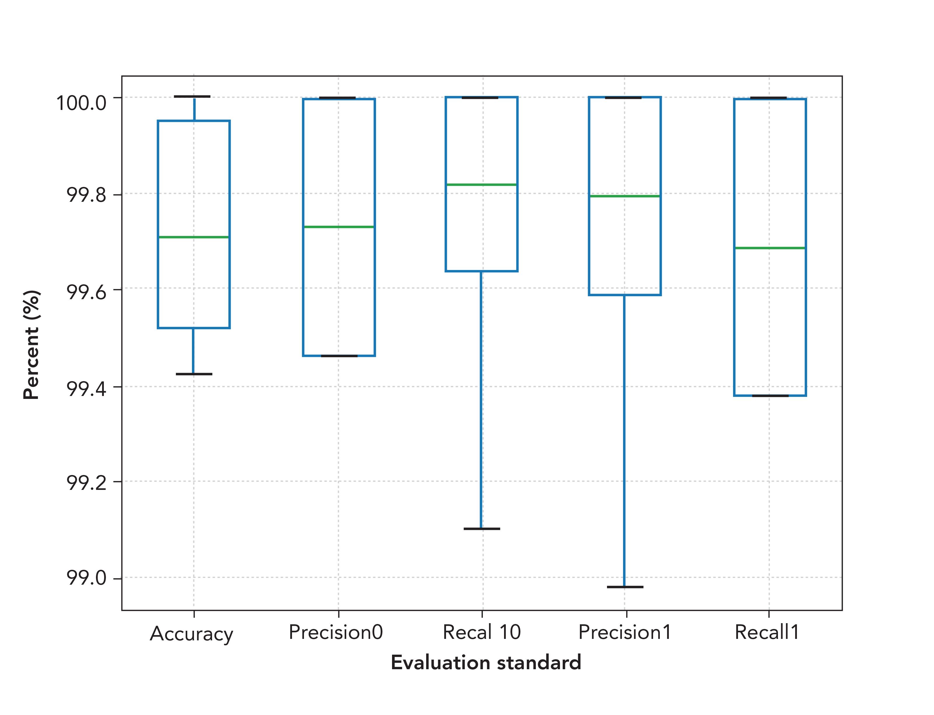
To evaluate the indicators of multiple experimental results in our model, we have conducted a third set of experiments. The results of 10 experiments were plotted into box plots, as shown in Figure 12. The overall average classification accuracy of 99.72%, precision0 of 99.73%, recall0 of 99.75%, precision1 of 99.71%, and recall2 of 99.69% were obtained.

FIGURE 12: Results of multiple experiments are shown in the box diagram. The green lines within the rectangles indicate the median, whereas the top and bottom ends of the rectangle represent the upper and lower quartiles, respectively.

Conclusion

In this work, a combination of WGAN and ResNeXt has been used to enhance and classify a small sample FT-IR spectrum dataset. The validity of this method has been proven by using the mean index of the evaluation criteria accuracy, precision, and recall. A combination of the classic dimensionality reduction algorithm with the classic classification algorithm is observed to improve the classification effect with an increase in the number of synthetic samples. In addition, because of the importance of FT-IR spectrum recognition in the field of food technology, feature selection no longer needs to rely solely on the analysis of chemical substances. Because the feature selection did not rely on precise domain knowledge from experts, the proposed supervised deep learning approach based on a small sample size holds the potential to provide effective solutions to problems involving a small sample size in various fields. This method adopted in this work greatly promotes the enhancement of spectral data and opens up a new technique of classification of spectral data.

Acknowledgments

This work was supported by the National Natural Science Foundation of China (NSFC) (No. 61765014); Reserve Talents Project of National High-level Personnel of Special Support Program (QN2016YX0324); Urumqi Science and Technology Project (No. P161310002 and Y161010025); and Reserve Talents Project of National High-level Personnel of Special Support Program (Xinjiang [2014]22).

Appendix A. Supplementary Data

The source code models are available at https://github.com/zhaoyinan629/mypro- ject.git.

References

(1) N. Cebi, C.E. Dogan, A.E. Mese, D. Ozdemir, M. Arıcı, and O. Sagdic, Food Chem. 277, 373–381 (2019). https://doi.org/10.1016/j.foodchem.2018.10.125

(2) M. Bağcıoğlu, M. Fricker, S. Johler, and M. Ehling-Schulz, Front. Microbiol. 10, 902 (2019). https://doi.org/10.3389/ fmicb.2019.00902

(3) A. Ghosh, S. Raha, S. Dey, K. Chatterjee, A.R. Chowdhury, and A. Barui, Analyst 144(4), 1309–1325 (2019). https://doi.org/10.1039/C8AN02092B

(4) J.F.R. Rochac, N. Zhang, J. Xiong, J. Zhong, and T. Oladunni, "In Data Aug- mentation for Mixed Spectral Signatures Coupled with Convolutional Neural Networks," paper presented at the 9th International Conference on Information Science and Technology (ICIST) in Hulunbuir, China, 2019, pp. 402–407.

(5) V. Varkarakis, S. Bazrafkan, and P. Corcoran, Neural Networks 121, 101–121 (2020). https://doi.org/10.1016/j.neunet.2019.07.020

(6) E.J. Bjerrum, M. Glahder, and T. Skov, Data augmentation of spectral data for convolutional neural network (CNN) based deep chemometrics. arXiv pre-print arXiv:1710.01927 (2017).

(7) Y.S. Perl, C. Pallacivini, I.P. Ipina, M.L. Kringelbach, G. Deco, H. Laufs, and E. Tagliazucchi, bioRxiv (2020). https://doi. org/10.1101/2020.01.08.898999.

(8) S.T.M Ataky, J. de Matos, A.D.S. Britto Jr, L.E. Oliveira, and A.L. Koerich, Data Augmentation for Histopathological Images Based on Gaussian-Laplacian Pyramid Blending. arXiv preprint arXiv:2002.00072, (2020).

(9) P. Liu, H. Yang, and J. Fu, In Marine Biometric Recognition Algorithm Based on YOLOv3-GAN Network (International Conference on Multimedia Modeling, Springer, 2020), pp. 581–592.

(10) H. Phan, I.V. McLoughlin, L. Pham, O.Y. Chén, P. Koch, M. De Vos, and A. Mertins, Improving gans for speech enhancement. arXiv preprint arXiv:2001.05532 (2020).

(11) A. Biswas, and D. Jia, "In Audio codec enhancement with generative adversarial networks," paper presented at the ICASSP 2020–2020 IEEE International Conference on Acoustics, Speech and Signal Processing (ICASSP) in Barcelona, Spain, 2020, pp. 356–360.

(12) C. Li, S. Anwar, and F. Porikli, Pattern Recognition 98, 107038 (2020). https://doi.org/10.1016/j.patcog.2019.107038.

(13) J. Liu, M. Osadchy, L. Ashton, M. Foster, C.J. Solomon, and S.J. Gibson, Analyst 142(21), 4067–4074 (2017). https://doi.org/10.1039/C7AN01371J.

(14) X. Zhang, T. Lin, J. Xu, X. Luo, and Y. Ying, Analytica Chimica Acta 1058, 48–57 (2019). https://doi.org/10.1016/j.aca.2019.01.002

(15) M. Fukuhara, K. Fujiwara, Y. Maruyama, and H. Itoh, Analytica Chimica Acta 1087, 11–19 (2019). https://doi.org/10.1016/j.aca.2019.08.064

(16) J. Acquarelli, T. van Laarhoven, J. Gerretzen, T.N. Tran, L.M. Buydens, and E. Marchiori, Analytica Chimica Acta 954, 22–31 (2017). https://doi.org/10.1016/j.aca.2016.12.010

(17) D. Nyasaka, J. Wang, and H. Tinega, Learning Hyperspectral Feature Extraction and Classification with ResNeXt Network. arXiv preprint arXiv:2002.02585 (2020).

(18) X. Zheng, G. Lv, Y. Zhang, X. Lv, Z. Gao, J. Tang, and J. Mo, Spectrochimica Acta A. 215, 244–248 (2019). https://doi.org/10.1016/j.saa.2019.02.063

(19) P. Koziol, M.K. Raczkowska, J. Skibinska, S. Urbaniak-Wasik, C. Paluszkiewicz, W. Kwiatek, T.P. Wrobel, Scientific Reports 8(1), 1–11 (2018). https://doi.org/10.1038/ s41598-018-32713-7

(20) X. Wang, S. Tian, L. Yu, X. Lv, and Z. Zhang, Lasers Med. Sci. (2020). https://doi.org/10.1007/s10103-020-03003-4

(21) I. Goodfellow, J. Pouget-Abadie, M. Mirza, B. Xu, D. Warde-Farley, S. Ozair, A. Courville, and Y.I. Bengio, Adv. Neural Inf. Process Syst. 9(2), 2672–2680 (2014).

(22) I. Gulrajani, F. Ahmed, M. Arjovsky, V. Dumoulin, and A.C. Courville, Adv. Neural Inf. Process Syst. 27, 5767–5777 (2017).

(23) R. Sharma, P. Halarnkar, and K. Choudhari, Kidney and Tumor Segmentation using U-Net Deep Learning Model. Available at SSRN 3527410, (2020). https://doi.org/10.2139/ssrn.3527410

(24) J. Liu, J. Wang, W. Ruan, C. Lin, and D. Chen, J. Med. Syst. 44(1), 15 (2020). https://doi.org/10.1007/s10916-019-1502-3

(25) K. He, X. Zhang, S. Ren, and J. Sun, "In Deep residual learning for image recognition," paper presented at the Proceedings of the IEEE conference on computer vision and pattern recognition in Las Vegas, Nevada, 2016, pp. 770–778.

(26) K. Simonyan and A. Zisserman, Very deep convolutional networks for large-scale image recognition. arXiv preprint arXiv:1409.1556 (2014).

(27) A. Krizhevsky, I. Sutskever, and G.E. Hinton, Adv. Neural Inf. Process Syst. 1, 1097–1105 (2012).

(28) C. Szegedy, S. Ioffe, V. Vanhoucke, and A. Alemi, Inception-v4, inception-resnet and the impact of residual connections on learning. arXiv preprint arXiv:1602.07261 (2016).

(29) C.F. Forney, W. Kalt, and M.A. Jordan, HortScience 35(6), 1022–1026 (2000).

(30) K. Fukuhara, X. Li, S. Yamashita, Y. Ha- vata, and Y. Osajima, "In Analysis Of Volatile Aromatics In ́ Toyonoka ́ Straw- berries (Fragaria × Ananassa) Using Porapak Q Column Extracts," paper presented at the 5th International Strawberry Symposium in Queensland, Australia, 2004, 708, 343–348.

(31) I. Zabetakis and M.A. Holden, J. Sci. Food Agric. 74(4), 421–434 (1997). https://doi.org/10.1002/(SICI)1097-0010(199708)

(32) D. Dong, C. Zhao, W. Zheng, W. Wang, X. Zhao, L. Jiao, Scientific Reports 3, 2585 (2013). https://doi.org/10.1038/srep02585

(33) M.I. Santos, C. Araujo-Andrade, E.E. Tymczyszyn, and A. Gómez-Zavaglia, Food Res. Int. 64, 514–519 (2014). https://doi.org/10.1016/j.foodres.2014.07.040

(34) G.F. Mohamed, M.S. Shaheen, S.K. Khalil, A. Hussein, and M.M. Kamil, Nature and Science 9(11), 21–31 (2011).

(35) L. Cassani, M. Santos, E. Gerbino, M. del Rosario Moreira, and A. Gómez-Zavaglia, J. Food Sci. 83(3), 631–638 (2018). https://doi.org/10.1111/1750- 3841.13994

(36) G. Teng, Q. Wang, J. Kong, L. Dong, X. Cui, W. Liu, K. Wei, and W. Xiangli, Optics Express 27(5), 6958–6969 (2019). https://doi.org/10.1364/OE.27.006958

(37) D. Zhu, L. Xu, X. Chen, L.-m. Yuan, G. Huang, L. Li, X. Chen, and W. Shi, Optics Express 28(12), 17196–17208 (2020).

Yinan Zhao and Shengwei Tian are with the College of Software Engineering at Xin Jiang University in Urumqi, China. Long Yu is with the Network Center at Xin Jiang University in Urumqi, China. Yan Xing is with the First Affiliated Hospital of Xinjiang Medical University in Urumqi, China. Direct correspondence to Shengwei Tian at the following email: tianshengwei@163.com.