Statistics and Chemometrics for Clinical Data Reporting, Part II: Using Excel for Computations

As described in the previous column (1), often there is confusion in multidisciplinary uses of statistical methods for analytical methods due to the variation in terminology, assumptions, and specific uses within different technical disciplines. Certain analytical methods of analysis are concerned only with overall error of analysis or correlation; others emphasize repeatability and reproducibility, and yet others report only bias and precision. Often, engineers look at total error analysis as tolerance stacking so that the sums of all errors in a specific dimension are less than the total maximum allowable tolerance.

As noted in Part I of this column series, a unification of multiple disciplines into a reasonable set of statistical parameters remains useful for a broad presentation of clinical analytical data. A single set of statistical parameters is useful to a multidisciplinary team involved in looking at analytical method comparison.

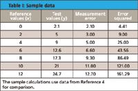
Table I: Sample data

This column describes the use of an Excel spreadsheet that computes and displays the statistical parameters described in Parts I and II of this series. For each parameter, the basic Excel computation nomenclature is described. The equations and terminology in this column are consistent with Clinical and Laboratory Standards Institute (CLSI) guidelines (2); please refer specifically to these guidelines referenced below for your own assessment. These statistical analyses evaluate the accuracy of a test method compared with a reference method measuring the same analyte.

Table II: Sample data in Excel format

Readers can refer to Part I of this column series for more detailed definitions of terms and to references 3–5 for additional descriptions and worked problems associated with the individual statistics demonstrated in this article. Note the data used for Parts I and II are shown in Tables I and II, and the entire Excel spreadsheet with computed results is shown in Table III. Also note the specific locations of data and calculations by rows and columns when referring to the Excel computation formulas.

Table III: Excel spreadsheet showing all calculations

Basic Definitions

A comparison of methods records differences between a test method and a comparative or reference method:

• X: comparative or reference method

• Y: test method

• x_i: observation i from comparative (reference) method

• y_i: observation i from test method

• n: total number of observations i

For clarity, this column assumes the comparative (reference) method is a traceable reference method that has better precision than the test method, which can be achieved by averaging replicate reference measurements if necessary.

Measurement Error

The measurement error (e_i) is the test method measurement minus the reference method

e = Test Measurement – Reference Method

or equivalently, using the CLSI definitions, the measurement error for the for the ith observation is

e_i = y_i – x_i

Accuracy

Accuracy includes both random and systematic components of a single measurement. Accuracy for a group of observations of the test method relative to the comparative method is calculated as

where n is the number of measurements.

Using Excel: ACCURACY =SQRT(SUM(E2:E8)/(COUNT(E2:E8)))

This calculation uses the error column represented by E2 through E8.

Trueness and Bias

Trueness is the closeness in agreement between the average value from a series of measurements and a recognized reference method or traceable standard. The measure of "trueness" is usually expressed in terms of bias (B):

Bias = average (Test Measurement) – average (Reference Method)

Using Excel: BIAS =AVERAGE(B2:B8) – AVERAGE(A2:A8)

Standard Deviation (As a Measure of Repeatability)

In blood samples, the glucose level can change due to red blood cell metabolism. If these glucose changes are a significant contribution to the standard deviation, then repeatability can be approximated from the measurement errors:

This is an approximation because the repeatability estimate now includes the imprecision of both the test method and the reference method.

Using Excel: SD =SQRT((SUM(E2:E8)–(SUM(D2:D8)^2/COUNT(A2:A8)))/(COUNT(A2:A8) –1))

The Excel formula can be simplified by using the EXCEL built-in function for Standard Deviation as follows: SD =STDEV(D2:D8)

Precision

Precision should be reported in absolute units (such as milligrams per deciliter) and in relative units expressed as a coefficient of variation. The coefficient of variation expresses the precision relative to the average reference value (x_i. mean).

Using Excel: CV% =G8/(AVERAGE(A2:A8))

Computation of the Regression Line

Coefficient of determination (R²): The coefficient of determination, R², is the square of the Pearson product-moment correlation coefficient. This statistic represents the amount of variation in the data that is modeled by linear fit of the test and comparative data pairs as a fraction of 1.0, as shown in Table III.

Using Excel: R2 =RSQ(B2:B8,A2:A8)

The correlation coefficient is the square root of R2 or

Using Excel: r =SQRT(M8)

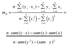
Slope (m₀): This is the slope of the regression line between x and y paired values. A slope of 1.00 indicates perfect agreement between a change in reference value magnitude and a change in test value magnitude. This slope value does not indicate the magnitude of the bias or of the intercept of the regression line between x and y values. It is computed as follows (summation notation is indicated):

Using Excel: SLOPE =SLOPE(B2:B8,A2:A8)

[Note: Equation 7 in Part I of this subseries had a typo in the right-hand side of the equation; this equation has been corrected, here.]

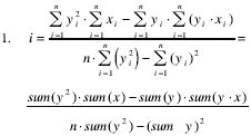
y-Intercept (i). The y-intercept is the point on the y-axis where the regression line crosses the 0 reference (x) value. It is not the bias, which has already been defined as Parameter 3. In summation notation the intercept is computed as follows:

Using Excel: INTERCEPT =INTERCEPT(B2:B8,A2:A8)

Linear Regression Corrected Results

The regression of Y on X from the data in Tables I and II results in a slope of 1.9304 and a bias of 1.5179 (shown in Table III); the linear regression equation using these data is as follows:

Generic form: Test Value (y_i) = Slope × (Reference Value, x_i) + BIAS

For our specific data: Test Value (y_i) = 1.9304 (Reference Value, x_i) + 1.5179

And so to compute the corrected test value (y^{^}_i) which corresponds to the reference value (x_i), we use the following equation:

Generic form: Corrected Test Value (y_i) = (Test Value (y_i) – BIAS)/SLOPE

For our specific data: Corrected Test Value (y_i) = (Test Value (y_i) – 1.5179)/1.9304

The Excel version for the corrected error for each value constituting the O column is as the reference value in the B column corrected as follows:

Using Excel: Corrected Test Values (y_i) =((B2)–1.5179)/1.9304

Note: The error (corrected) and standard deviation (corrected) are calculated using the same formulas as before, only for the bias and slope corrected errors, as shown in Table III, column O. If a global or universal bias and slope are known to exist between the comparative (reference) method and the test method, then the correction using bias and slope using these global values is warranted.

Acknowledgment

We would like to thank Drs. Bill Patterson, Shonn Hendee, Stephen Vanslyke, and David Abookasis of Luminous Medical for their multidisciplinary contributions. in authorship, review, and editing.

Howard Mark serves on the Editorial Advisory Board of Spectroscopy and runs a consulting service, Mark Electronics (Suffern, NY), hlmark@prodigy.net.

Jerome Workman, Jr. serves on the Editorial Advisory Board of Spectroscopy and is currently with Luminous Medical, Inc., a company dedicated to providing automated glucose management systems to empower health care professionals.

References

(1) J. Workman, and H. Mark, Spectroscopy 24(6), 18–20 (2009).

(2) Clinical and Laboratory Standards Institute (CLSI) guidelines: Q300-001, Terminology for standard definitions. For more details on statistical estimation and verification see:

• CLSI Document EP5-A2, Evaluation of Precision Performance of Quantitative Measurement Methods; Approved Guideline – Second Edition.

• CLSI Document EP10-A2, Preliminary Evaluation of Quantitative Clinical Laboratory Methods; Approved Guideline – Second Edition.

• CLSI Document EP15-A2, User Verification of Precision and Trueness; Approved Guideline – Second Edition.

• CLSI Document EP9-A2, Method Comparison and Bias Estimation using Patient Samples; Approved Guideline – Second Edition.

• CLSI Document EP10-A2, Preliminary Evaluation of Quantitative Clinical Laboratory Methods; Approved Guideline – Second Edition.

• CLSI Document EP15-A2, User Verification of Precision and Trueness; Approved Guideline – Second Edition.

(3) W.J. Youden and E.H. Steiner, Statistical Manual of the AOAC, 1st ed. (Association of Official Analytical Chemists, Washington, D.C., 1975).

(4) J.C. Miller and J.N. Miller, Statistics for Analytical Chemistry, second ed. (Ellis Horwood, New York, 1992).

(5) H. Mark and J. Workman, Chemometrics in Spectroscopy (Elsevier/Academic Press, Boston, 2007), Chapters 58–61.