Detection of Early Bruises in Honey Peaches Using Shortwave Infrared Hyperspectral Imaging

Honey peaches can bruise during harvesting, handling, storage, transportation, and distribution. In this study, the spectral range used was 400–1100 nm, and we extracted the RGB and HSI color space characteristics of the images. After principal component analysis (PCA) of the original data, the gray histogram features of the PC1 images were extracted. Partial least squares qualitative discriminant analysis (PLS-DA) and extreme learning machine (ELM) discriminant models were established. Among the 38 color features, the PLS-DA and ELM models had a high rate of misclassification, and the best classification accuracy was 74.29%. When extracting the spectral information of the bruised sample to build the model, the highest classification accuracy was 92.86% for the 176 characteristic wavelength points of the full band. In contrast, only 40 wavelength bands were used after selecting the genetic algorithm’s valid information. The classification accuracy of the PLS-DA model was 100%, which is because the softening and browning of the peach was not apparent after early bruising. However, the changes in the tissue’s thermal properties caused by internal defects are expressed in the internal spectrum. Therefore, the shortwave NIR hyperspectral imaging technique’s spectral information can detect the early bruising of peaches.

Honey peaches are one of the most critical economic fruits in the world. China has the largest peach plant area and the largest production scale compared to other countries such as Italy, Greece, Spain, and the United States (1). From a nutritional perspective, honey peaches are a good source of dietary fiber, vitamin B, vitamin C, carbohydrates, minerals, organic acids, folic acid, and dietary antioxidants. The protein content of honey peaches is twice that of apples and grapes and seven times higher than pears. The iron content is three times higher than apples and five times higher than pears (2). The presence of bruise defects is one of the most influential factors in the quality and price of a honey peach. In general, customers pick up a honey peach and judge its quality by external attributes such as shape, color, and size. A moderate amount of bruising often deters consumers from purchasing a peach, which can lead to postharvest loss and an overall decrease in profits across the industry. Moreover, honey peaches affected by bruises will tend to ferment, decay, and infect other non-bruised peaches after damage. However, naked eye observations are limited in evaluating peach bruising. Moreover, efficiency and accuracy would be significantly reduced after continuous manual inspection. Therefore, it is essential to develop a rapid, non-contact detection technique to identify the honey peach bruising and determine its bruise degree. By sorting honey peaches following their bruise degrees, it would result in higher quality peaches hitting the market, which means better prices and less food waste, increasing profits (3,4).

Hyperspectral imaging is an emerging technique in recent years that can provide both spatial and spectral information. During hyperspectral imaging analysis, the spectra are used as a fingerprint to identify and measure the vibration in energy absorption that depends on the sample’s chemical composition and moisture content. In general, machine vision technology based on a red, green, and blue (RGB) color camera is more effective for detecting those bruises (5). Hyperspectral imaging also has potential in detecting bruises in various fruits, including peaches. Hyperspectral imaging integrates conventional imaging and spectroscopy to provide both the spatial and spectral information of an object. Each hyperspectral image contains a large amount of information that can be analyzed to characterize the object more reliably than the traditional machine vision technology (6–10). A few characteristic wavelength images could be selected to develop rapid multispectral imaging systems for fast bruise detection. It is advanced and efficient to detect non-obvious bruises of samples and assess internal attributes of fruits. Keresztes and others used hyperspectral imaging to detect the varieties and bruises of apples, and the correct rate of the classification of varieties and bruises reached 96% and 90.1%, respectively (11). Lopez-Maestresalas and others studied potato bruises in the visible-near-infrared (vis-NIR) and shortwave NIR wavelength ranges, with a classification accuracy rate of 98.56%, showing that early bruises can be detected on food items (12). Vetrekar and others verified the feasibility of nondestructive testing of apple, heart fruit, and guava fruit bruises in the wavelength range of 400–1000 nm (13). Zhang Baohua and others used hyperspectral imaging combined with the minimum noise separation algorithm (MNF) to detect minor bruises with an accuracy rate of 97.1% (14). Wu Longguo and others used hyperspectral imaging to study the various defects of Lingwu Changzao jujubes and insect eyes, and the accuracy rate of various defects reached more than 86% (15). Jiangbo Li and others used longwave and shortwave NIR hyperspectroscopy combined with an improved watershed algorithm to analyze early peach bruising and obtained excellent results, laying a foundation for the study of early peach bruising (16). These reports show that NIR hyperspectral imaging combined with the appropriate detection algorithms can effectively identify bruised fruit.

Partial least squares (PLS) regression is the most widely used algorithm in the process of solving the linear relationship between hyperspectral imaging and target data (17). Extreme learning machine (ELM) has many unique advantages in solving small sample, nonlinear, and high-dimensional pattern recognition. ELM has a reduced computational complexity (18). Variable selection is another critical factor affecting the accuracy of a prediction model. To improve the accuracy and robustness of the prediction model, the compensation model of biological or environment variability was built with variable selection tactics. The selection of characteristic wavelength can eliminate the collinearity, redundancy, and noise in the full wavelength spectrum, thus improving the prediction accuracy, which involves many variable selection algorithms. However, the results obtained from different variable selection algorithms are usually different because of their varied principles and applications (19,20).

The accuracy of fruit bruise detection is influenced by many factors, such as the variety of bruises, location, severity, fruit variety, and storage time. Some can be detected directly by image segmentation, but some of the minor bruises cannot be observed by machine vision technology. It is necessary to analyze the mechanism of fruit bruising, taking into account changes in the internal spectrum of the fruit in question. In previous studies, it has been suggested that shortwave NIR is sufficient to distinguish the early bruising of peaches (21). This study started with using simplified equipment. It only used the hyperspectral shortwave camera to collect sample information and further analyze the results (22,23). The aims of this study were to: 1) extract the characteristics of the image of the sample, including the RGB, HSI color characteristics, and gray histogram statistical characteristics of the model; 2) compare the spectral features of sound peaches and bruised peaches, and mechanically find out the differences between sound peaches and bruised peaches; 3) compare the six detection results produced by the two algorithms using image feature information, full-band spectral information, and the influential band of the spectra selected by the genetic algorithm (GA) as input values of the prediction model, respectively; and 4) draw conclusions for distinguishing bruised peaches from uninjured tissues and provide a theoretical basis for online fruit bruise detection.

Materials and Methods

Sample Preparation and Bruise Treatment

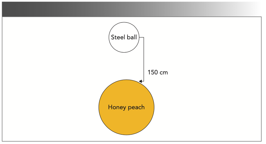
The experimental sample selected in this study was the honey peach, and the peach variety was Yangshan. Figure 1 shows a picture of the experimental sample. To prevent other factors from affecting the experimental results, the samples’ size and weight remained identical. The equatorial diameter of the honey peach was 80 ± 5 mm; all models were carefully selected before the experiment to ensure that the samples’ appearance was free from defects and damages. The bruised parts were chosen near the equator of the honey peach. The number of experimental models was 210, of which 120 were injured and 90 were undamaged. A steel ball was used to obtain the bump sample and form a bruise. The mass of the steel ball was 33 g, the diameter of the steel ball was 20 mm, and it was placed 160 mm above the surface of the honey peach. Then, the free-fall motion was performed, and a bump sample was formed by hitting the equator of the honey peach. Finally, the 210 pieces were placed in an environment with a room temperature of 24 °C and relative humidity of 65%, and the image was collected 1 h later. The purpose of standing for 1 h was to keep the sample temperature consistent with the ambient temperature. Figure 2 shows a schematic diagram of the simulated impact (16).

FIGURE 1: Picture of the experimental sample.

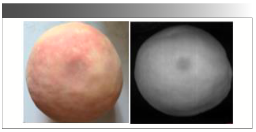
FIGURE 2: Schematic diagram of the bruise simulation.

The left of Figure 1 shows the intact sample, and the right shows the slight bump in the piece. The total number of samples is 140, 70 samples are used for modeling and the remaining 70 samples are used to validate the model. The number of pieces in the prediction set was used to evaluate the model.

Hyperspectral Imaging System and Data Acquisition

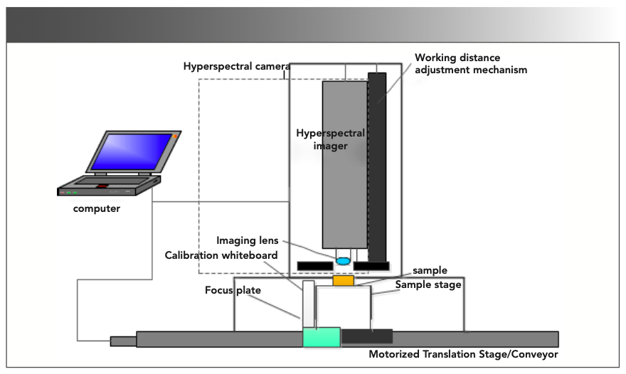
The hyperspectral imaging system included a light source, an imaging spectrometer, a charge-coupled device (CCD) camera, a lens, a displacement platform, a controller, a dark box, and a computer. The spectral resolution was 2.8 nm, and the spectral range was from 380 to 1080 nm. As shown in Figure 3, a schematic diagram of the structure of the hyperspectral imaging system is shown. The camera exposure time was 20 ms, the interval of spectral radiation energy was approximately 2.4 nm; the platform travel speed was approximately 15 mm/s. Because the image acquisition process was susceptible to the effects of ambient light, the entire imaging system was placed in a confined space to eliminate the influence of ambient light, which prevented the effects of natural light and improved the quality of the acquired data.

FIGURE 3: Diagram of the hyperspectral imaging system.

Because of the spatial intensity change of the halogen lamp on the acquisition plane, a dark current also existed in the CCD camera. These factors interfered with specific wavebands and affected the quality of the image. Therefore, before data processing, the data needed to be corrected in black and white. The calibration process was completed on the SpecView software. First, the lens was aimed at the whiteboard before the whiteboard button was clicked to collect the whiteboard image and background information. To prevent the lens from rotating and causing the focal length to change, the lens was held sideways to screw on the lens cover. Once that step was completed, the blackboard button was clicked to collect the blackboard image. The black and white correction was based on equation [1] below:

In equation [1], R_xy(λ) is the raw image data; R_dark(λ) is the all black calibrated image data; R_white(λ) is the all white calibrated image data; and I_xy(λ) is the black and white corrected image data (24,25).

Data Processing and Analysis

Principal Component Analysis (PCA)

Principal component analysis (PCA) enhances the information content of hyperspectral images and has the advantages of isolating noisy signals and reducing the dimensionality of the data. It is possible to comprise previously redundant information into manually irrelevant data, while at the same time replacing all of the spectral information with less information in a practical sense. The algorithm works on the following principle: suppose a given training data set contains N samples X, XєRⁿ, X is for each sample: X₁ = [x_I1, x_I2,...,x_ln]^TєRⁿ. The mean value of X is m and the covariance matrix of the training set is as follows:

The eigenvalue of Σ represents the distribution variance of the sample on the eigenvector.

Select d eigenvectors of Σ and sort them according to the eigenvalues. The dimensionality reduction feature subspace is expressed as YєRd,d<<n:

Y1 = {y_1l, y_2l,...y_dl} (26).

Genetic Algorithm (GA)

The GA has its origins in the study of computer simulations of biological systems. It is a stochastic global search and optimization method developed to mimic natural organisms' evolutionary mechanisms, drawing on Darwin's theory and Mendel's theory of genetics. It is essentially an efficient, parallel, and global search method that automatically acquires and accumulates knowledge about the search space during the search process and adaptively controls the search process to find the best solution. This study uses the genetic algorithm to select spectrally valid information, reducing the number of model calculations while improving model detection accuracy.

Partial Least Squares Discriminant Analysis (PLS-DA)

The partial least squares linear discrimination analysis (PLS-DA) method is a regression model that can establish the relationship between sample categorical variables and spectral characteristics. Sample classification variables are used instead of sample variables. The linear relationship between the statistical classification variables and the spectral matrix was used to establish a qualitative discrimination model. The calculation steps of peach spectrum X and bruising time Y between T and U are shown in equations [5] and [6]:

T and U are the score matrices of X and Y, respectively; P and Q are the load matrices of X and Y, respectively; and E and F are the PLS fitting residual matrix of X and Y, respectively. The linear regression equations of T and U are equations [7] and [8]:

where B is the correlation matrix. The score array T of the unknown sample is obtained from the spectral array X and the load array P. Then, the collision time of unknown samples can be calculated according to equation [9]:

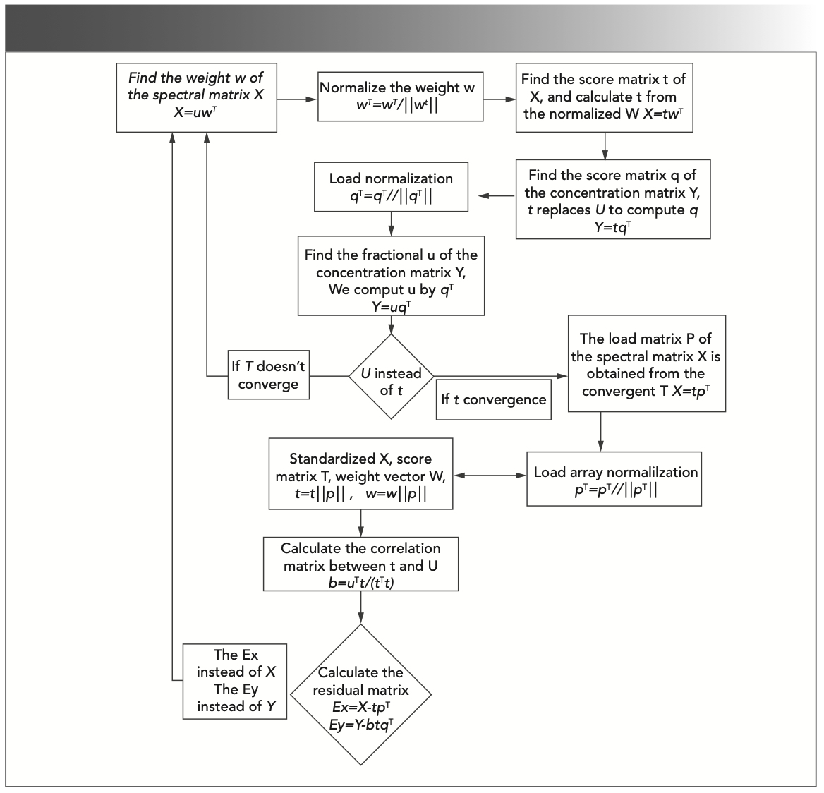
The flow chart of calculation during modeling is shown in Figure 4, and the corresponding matrix factors w, t, p, u, q, and b can be obtained.

FIGURE 4: The modeling calculation flowchart.

During the prediction period, the predicted value of unknown samples can be calculated according to equation [10]:

where y = b_KX_unknownb_K = w^T (pw^T)^-1q is the regression coefficient (27,28).

ELM

ELM is a single hidden layer feed forward network with random input weight selection and output weight estimation analysis, assuming that in the flow chart of ELM algorithm, X is the input variable; G(x) is the excitation function; w is the weight variable that connects the implicit node to the input node; b is the offset of the implicit node; β is a weight variable that connects the implicit node to the output node; and f(x) is the output variable.

N sample spectra and actual values form a matrix of D rows and m columns, whereas the excitation function and hidden node L are mathematically obtained by equation [11]. The predicted results can be calculated by equation [12] (29–32).

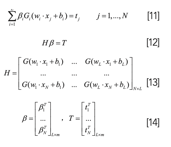
The implied node number L is determined randomly, while the weight of the β matrix is estimated by ß(ß=H^TT), and β can also be estimated by ß=(H^TT+λI)^-1H^TT to obtain a stronger generalization performance. The conventional parameter was λ > 0, so the global optimal solution was obtained by analyzing the ELM output weight, avoiding the complicated convergence problem in the early stage (33,34).

Spectral Feature Extraction

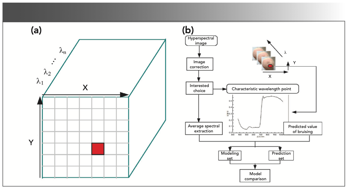
The sample spectral feature extraction was performed with the envi4.5 software to ensure that the selected sample spectrum was representative, prevented the single-pixel point spectrum from the overall spectral difference of the sample, and failed to express the correct information of the model. The sample spectral feature was considered the average range of the area of interest. After reading the sample image, the region of interest (ROI) in the rectangular area was selected. The image data obtained by hyperspectroscopy is a “three-dimensional (3D) data block,” in which X and Y represent two-dimensional plane pixel information coordinates. The third dimension is the wavelength information coordinate axis. The number of pixels in the region of interest was selected to be 100, and the average spectrum of 100 pixels was calculated. Figure 5 shows the ROI schematic diagram of the area chosen and the ROI selection process.

FIGURE 5: The region of interest selection diagram: (a) ROI schematic diagram of the selected area and (b) the ROI selection process.

Results and Discussion

Overview of Spectra and Images

To ensure that the spectra of the pieces were chosen to be representative and to prevent the scopes of individual pixels from differing significantly from the overall range of the sample, the spectral features of the pieces chosen were the average spectrum of the region of interest. After reading the sample image, a rectangular area of interest was selected. The number of pixels in the selected region of interest was 100, and the average spectrum of the 100 pixels was calculated.

Figure 6 shows a comparison of the reflection spectra of the bruised and the sound (unbruised) sample. The abscissa is the wavelength range of the spectrum, and the ordinate is the reflectivity. The image of the bruised piece at the wavelength of 810 nm was extracted, and the pseudo-color image was processed. Figure 6 contains the single-wavelength point’s grayscale image and the pseudo-color image of the bruised sample. One of the gray values increased gradually from blue to red because of the influence of the wild peach surface radian. The edge of gray value was lower than that near the middle of the room, which means that it is difficult to segment the damaged area, so only using single wavelength point of an image is difficult in identifying mild bruising (35,36).

FIGURE 6: Spectral comparison of damage and intact samples.

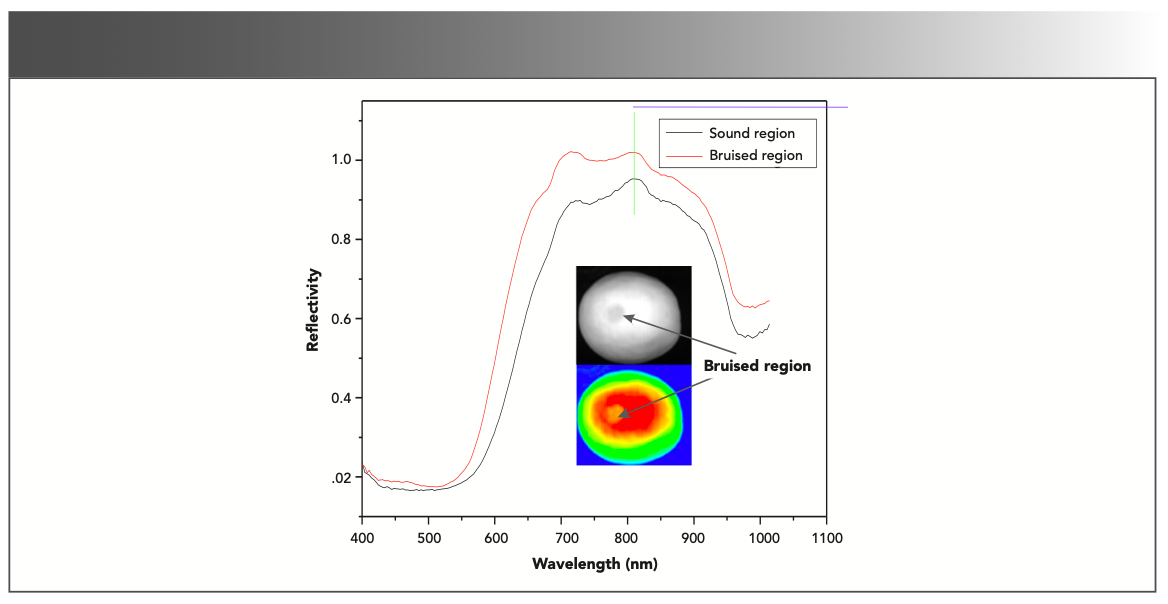
The average spectra of the bruised and normal regions of yellow peaches were extracted, and comparative analysis revealed that the waveforms of the two spectra had similarities, with absorption peaks at 714 nm, 815 nm, and 970 nm. This may be caused by the second overtone of the C-H functional group (37). The absorption peaks appearing at 815 nm and 970 nm wavelength points may be caused by the O-H and N-H functional groups. The spectral differences between the bruised and normal regions of yellow peaches are also related to differences in moisture content and other organic molecules (38–40).

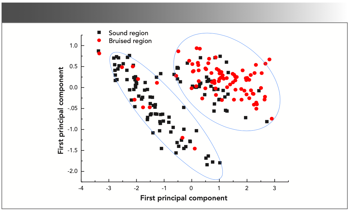
A scatter plot of the classification of bruised and sound peach data is shown in Figure 7. Black dots indicated a good peach, and the red dots indicated the bruised peach. The results show that there was clustering between the sound and bruised samples. It can be observed in the Figure 7 that the clustering phenomenon occurs between good peaches and bruised pieces. This phenomenon indicated that differences in the internal physiological parameters between post-bruise and sound samples could be detected spectroscopically or graphically. However, there is a partial crossover between post-bruise data and sound peach data, which makes it somewhat difficult to distinguish between grades and, as a result, requires further data analysis.

FIGURE 7: Scatter plot of bruised and Soung honey peach classification.

PCA in Wavelength Ranges

Using the shortwave NIR wavelength range (400–1100 nm), the peach bruises on the early samples were obtained by PCA. The high spectral reflection image of the first five images, as shown in Figure 8, represent the real PC images, to make the exact comparison of the different PC image corresponding to the pseudocolor images. As a general note, the original without the hyperspectral image change contains more information than the PC images, so the PC images have a certain degree of distortion and cannot keep the characteristics of the original image. As shown in Figure 8, the PC2 and PC4 images reveal no useful information. However, PC3 and PC5 show the bruised image contrast between the intact and damage tissue better; on the downside though, PC3 and PC5 contain segmentation errors because of the excessive area. PC3 also has a “false positive” error. Although PC1 is fuzzy, it retains the information that the image needs to be expressed. Therefore, the PC1 image was selected for the feature extraction.

FIGURE 8: Pictures of principal component analysis.

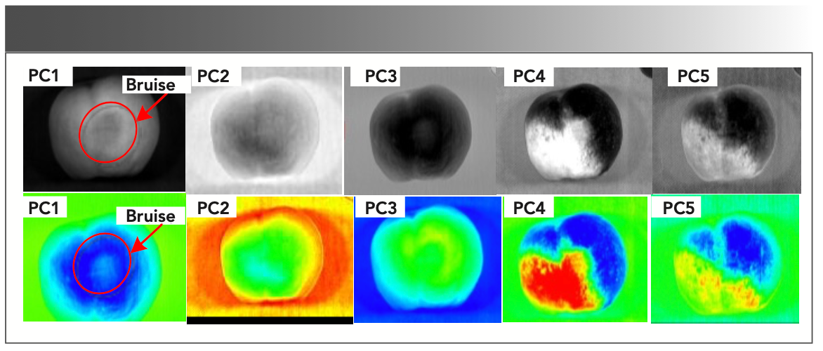
Image Feature Extraction

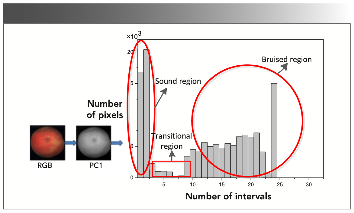
The main image features commonly used are color features, texture features, shape features, and spatial relationship features. The image features in this study refer to the color features of an image. After the fruit is bruised, the bruised area gradually changes color over time, becoming darker, and finally, black. Therefore, of all the image features, the color features are better suited to characterize the changes in the surface of the fruit after a bruise. Because of the change in color after a bruise, this change can be represented in the grayscale histogram of the image. In this study, color and gray histogram statistical features were chosen to characterize the sample image after bruising. The grayscale histogram statistical features refer to the occurrence times of corresponding pixel points in each cell of the grayscale image. The grayscale value range of the grayscale image was 0–255, and the interval selected in this study was eight. The interval range of 0–255 was divided into 32 cells, and the occurrence times of the corresponding pixel points in each cell were counted. It is important to note that in the gray-scale histogram of a multispectral, not all PCs have the same contrast (for example, in PC3, the sound and bruised areas have similar gray levels, so if the damaged areas with higher gray values are successfully segmented based on the PC3 images, this will result in a large number of sound tissues with lower gray values being misclassified).

As shown in Figure 9, the gray histogram of the PC1 image was extracted; the gray histogram was also an essential feature of the image, reflecting the relationship between the frequency of each gray level pixel and the gray level of an image. The abscissa was the interval number, which was divided into 32. As the interval number increased, the color components became lighter, and the smaller the interval value was, the darker the color was. The ordinate is the number of pixels. Figure 9 shows the bruising, sound, and transfer area. The larger the bruising size is and the higher the pixel point is, the more sensitive the bruising is in image statistics.

FIGURE 9: Gray histogram statistical feature extraction process.

Early Bruise Analysis of Peach with Hyperspectral Image Information

In this study, two color features, RGB and HSI, and 32 features from the sample’s grayscale histogram statistics, were extracted. The RGB color space is comprised of red, green, and blue components. In the RGB color space, the color of arbitrary F can use the following formula:

R, G, and B are the three color components of red, green, and blue, respectively, and the percentages of the three colors. Other colors in the RGB color space can be expressed through equation [15]. Extract the three-channel component of the whole sample, and then calculate the average value of the three-channel element respectively, as shown in the following formula:

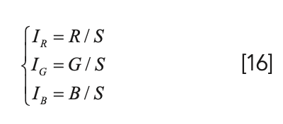
where I_R, I_G, and I_B are the mean values of the colors of the red, green, and blue channels, respectively; S is the number of pixels; and red, green, and blue are the color values of the three channels, respectively. Equation [16] can calculate the mean value of the color component of the RGB three-channel of the image and use it as the final modeling data. However, I_H, I_S, and I_l can realize the conversion from RGB color space through equation [17].

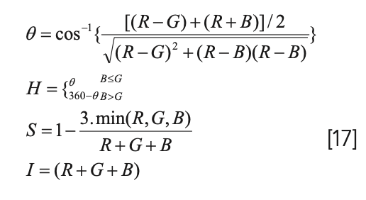
A total of 38 valid features were input, and the average values of the three channel components of each color space, I_R, I_G, I_B, I_H, I_S, and I_I, were selected for modelling. All color features needed to be synchronized prior to building the detection model to reduce differences between the inputs. With 38 color features as the inputs, the bruised peaches set to 1, and the good peaches set to 0, there were 70 ones and 140 zeros in the total data. A regression model with qualitative discrimination between a matrix of 210 multiplied by 38 and 210 set values, which in turn contained the PLS and ELM models. Of the 210 samples, 140 of them were randomly selected as the modeling set. The remaining 70 pieces were used as the prediction set. Table I shows the early bruise area discrimination results for honey peaches based on the hyperspectral water image information, with a lower false positive rate that indicates a better model. The PLS discriminant model results show that 18 prediction sets were misclassified with a classification accuracy of 74.29%. The ELM discriminant model for the hardlim function had 26 misjudgments and only 62.86% were correct, the sigmoidal function has 22 misjudgments, the correct rate of classification is 68.57%, and the sine function was only 72.86% accurate for classification.

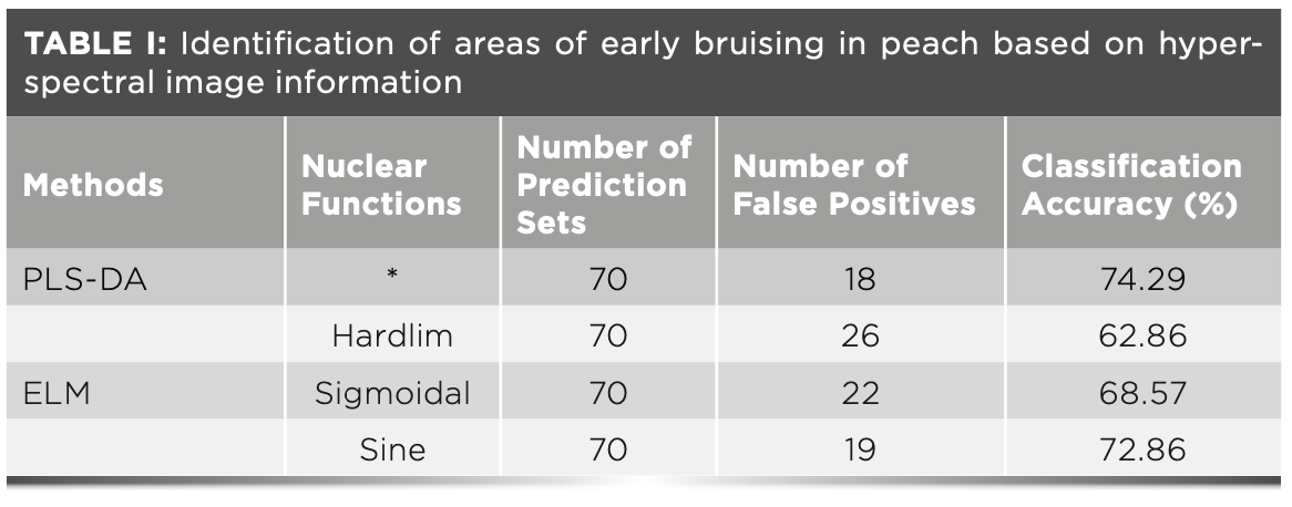
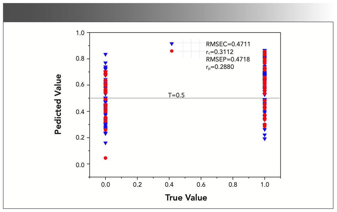
Figure 10 shows the effect diagram of image feature modeling: the red represents the modeling set, and the blue represents the prediction set. The threshold T was set at 0.5. When the value was less than 0.5, it was judged as a sound honey peach; when the value was more significant than 0.5, it was regarded as a bruised honey peach. The PLS-DA model established has a better classification effect than the ELM model. The RMSEC root mean square error of the modeling set (which was PLS-DA) was 0.4711, the correlation coefficient of the modeling set was 0.3122, the RMSEP of the prediction set was 0.4718, and the correlation coefficient of the prediction set was 0.2880.

FIGURE 10: Plot of PLS-DA image feature modelling results.

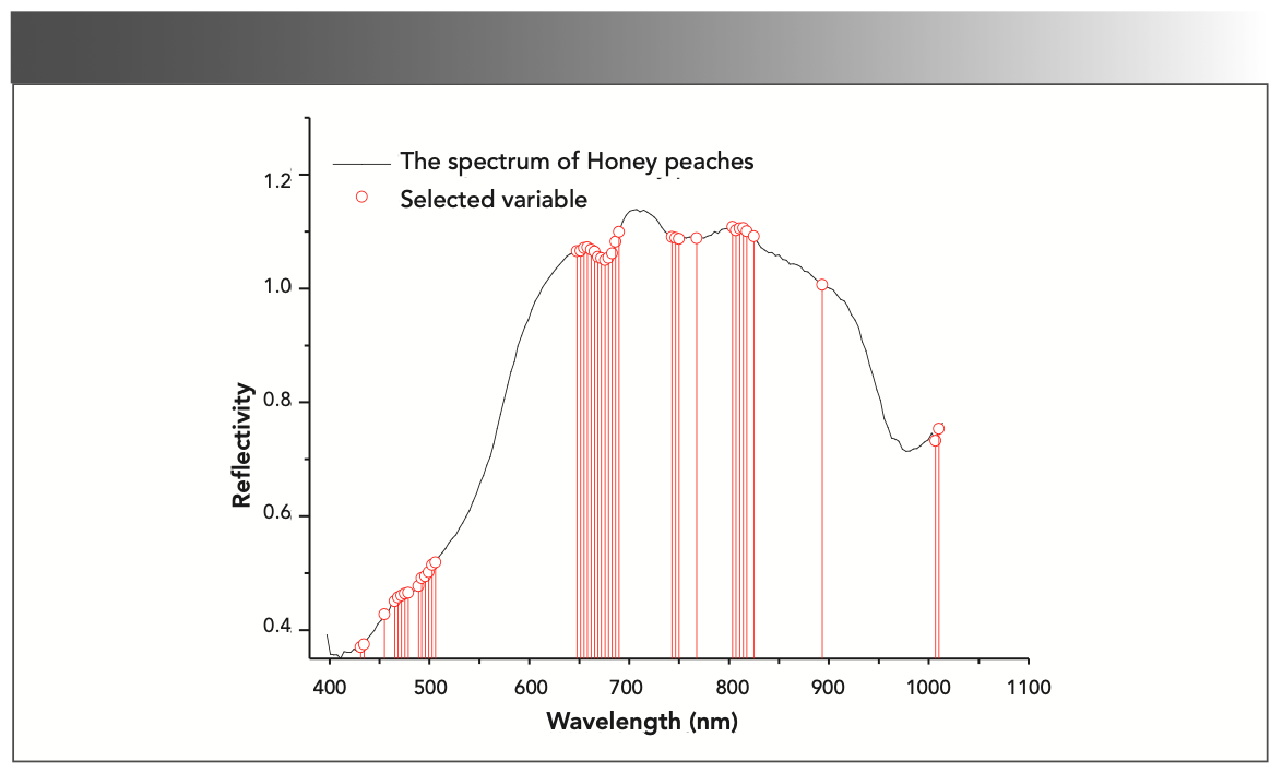
Spectral features in the 400–1100 nm wavelength range contain 176 characteristic wavelength points to better predict honey peach bruising early on. The genetic algorithm (GA) has a unique advantage in choosing its useful spectral bands, as shown in Figure 11. GA selected the adequate information of spectra, with a total of 40 useful wavelength points: 120, 81, 24, 30, 83, 175, 32, 80, 82, 84, 23, 119, 121, 85, 102, 31, 79, 25, 11, 101, 122, 22, 174, 12, 76, 118, 74, 77, 18, 21, 28, 143, 29, 124, 33, 78, 86, 103, and 104.

FIGURE 11: Genetic algorithm (GA) filtering spectrally valid information.

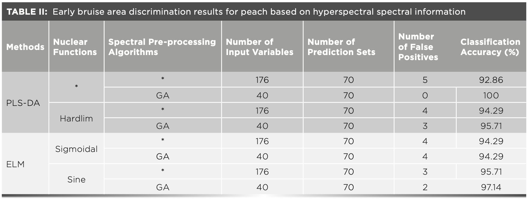
As shown in Table II, the early discriminant model for honey peach bruising was based on spectral information. The model input information included full-wave information and valid information selected by the GA. The PLS-DA model is shown in Table II. Five misjudgments occurred when the full band information was used as input, with a classification accuracy of 92.86%. After the GA picked the variables, the number of false positives in the 70 prediction sets was zero with a 100% classification accuracy rate. ELM is a new machine learning algorithm based on a single-hidden layer neural network. The input weights and offset numbers are randomly selected. The initial value of ELM hidden layer neurons is 10, and the step size is set to 1, which gradually increases to the number of modeling samples. In the training, the sigmoidal, sine, and hardlim functions were used as excitation functions of neurons, and the number of spectra was used as the input. Table II shows the modeling results of the three excitation functions. As can be seen from Table II, when sine was the excitation function, the classification accuracy was the best. When the whole spectral data was used as the input, only three samples had misjudgment. When the data after variable selection was used as the input, only two data points had misjudgment, and the classification accuracy was 97.14%.

The discriminant results of the PLS model are plotted in Figure 12, with a model set RMSEC of 0.1306, a modeled set correlation coefficient of 0.928, a modeled set RMSEP of 0.1357, and a predicted set correlation coefficient (r_p) of 0.928. The results for the PLS model is shown in Figure 12.

FIGURE 12: Graph of spectral feature modelling results.

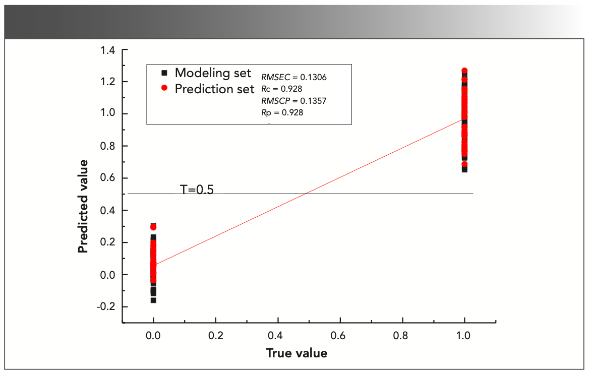
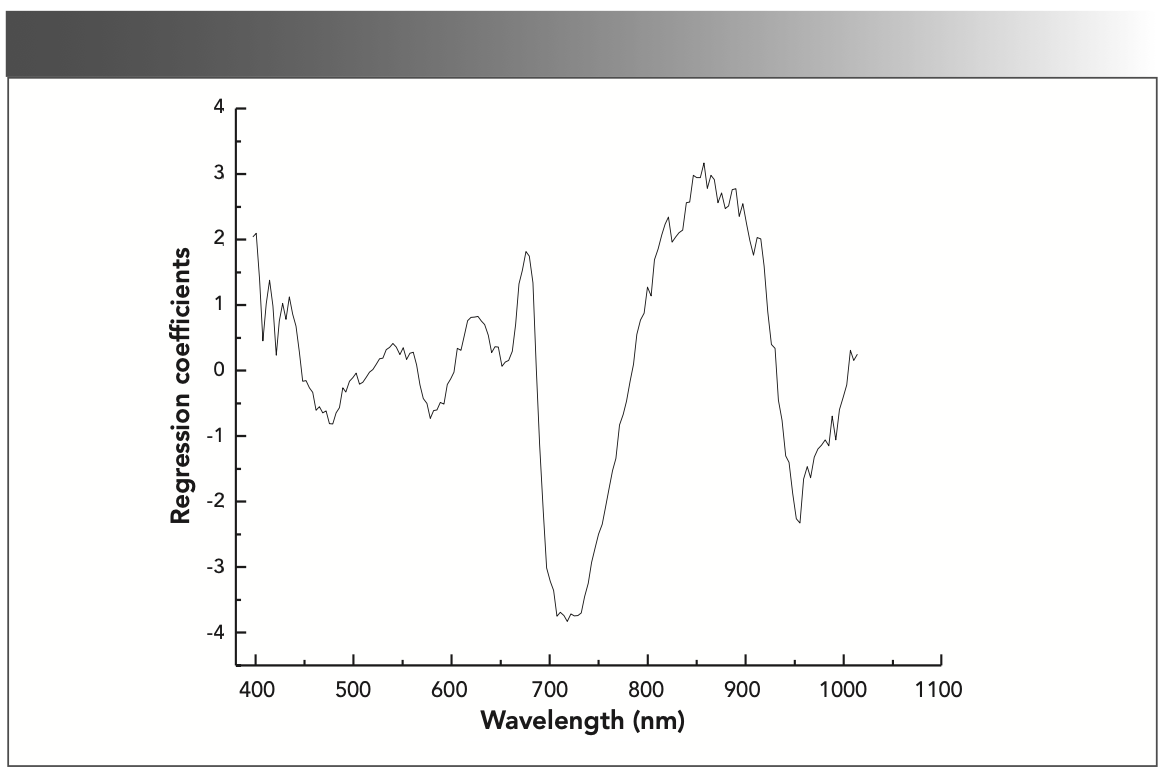
Figure 13 shows the predicted regression coefficients at different times after the bruising of the caper. The greater the weight of the spectral variables in the quantitative PLS model, the greater the regression coefficients. The greater the regression coefficient corresponding to the spectral variable, the more significant the contribution of the sample information to the model prediction.

FIGURE 13: Regression coefficient curves for the PLS-DA model.

Conclusion

This study demonstrated the high potential of hyperspectral imaging coupled with multivariate analysis to determine honey peach bruising. The PLS-DA regression model and the ELM regression model were used to establish the honey peach microjudgment discrimination model. In this study, based on the analysis of internal spectral features and external color features of bruised honey peach, the PLS-DA algorithm and ELM algorithm were used to establish the peach’s slight bruising discrimination model. The highest classification accuracy of color features was only 74.29%. In the spectral information analysis of the honey peach collision, the GA was used to virtually screen 176 spectral features. The PLS-DA model established based on the spectral all-band information was superior to the ELM model. After the GA selected 40 useful variables, there was no wrong number of samples in 70 prediction sets, and the classification accuracy was 100%. RMSEP was 0.1357, and the r_p was 0.928. The spectral information and image information were used as model inputs separately, and the model built by the spectral information was better than the image information. The reason may be because the softening and browning of internal tissues are not obvious after bruising of yellow peaches, and it is difficult to distinguish them in terms of appearance and color. The high accuracy of spectral information discrimination may be that the changes in thermal tissue characteristics caused by internal defects and physiological disorders are expressed through internal spectra. According to the spectral information, when the honey peach was slightly injured, the honey peach can still achieve its highest classification accuracy. In particular, online sensors will also be developed for honey peach sorting or post-harvest quality processing of other fruits.

Conflicts of Interest

There are no conflicts to declare.

Acknowledgments

The research was funded by the National Natural Science Foundation of China (No. 31760344), the Science and Technology Research Project of Education Department of Jiangxi Province (Grant No. GJJ200652), and the Science and Technology Research Project of the Education Department of Jiangxi Province (Grant No. 190306).

Author Contributions

Conceptualization was done by Xiong Li; the data curation was performed by Xiong Li and Guantian Wang. Funding acquisition for the study was handled by Xiong Li and Yande Liu; Xiong Li and Yunjuan Yan handled the writing, editing, and review of the manuscript.

References

(1) Q. Liu, P. Weng, and Z. Wu, Int. J. Food Prop. 23(1), 445–458 (2020).

(2) Y. Liu, Y. Zhang, and X. Jiang, Vib. Spectrosc. 111, 103152 (2020).

(3) Y.Y. Shao, G.T. Xuan, and Z.C. Hu, PloS One 14(9), 1–13 (2019).

(4) J.B. Li, LP. Chen, and W.Q. Huang, Postharvest Biol. Technol. 135, 104– 113 (2018).

(5) Y.D. Liu, M.J. Chen, and Y. Hao, J. East China Jiaotong Univ. 35(4), 1–7 (2018).

(6) G. ElMasry, C. Vigneault, and J. Qiao, Lwt - Food Sci. Technol. 41(2), 337–345 (2008).

(7) J.P. Cruz-Tirado, J. Pierna, and H. Rogez, Food Control 118, 107445 (2020).

(8) S.H. Park, Y.K. Hong, and S.B. Mubarakat, Spectrosc. Spect. Anal. 40(4), 319–324 (2020).

(9) K.B. Walsh, J. Blasco, and M. Zude-Sasse, Postharvest Biol. Technol. 168, 111246 (2020).

(10) E. Arendse, O.A. Fawole, and L.S. Magwaza, J. Food Eng. 217, 11–23 (2017).

(11) J.C. Keresztes, E. Diels, and M. Goodarzi, Postharvest Biol. Technol. 130, 103–115 (2017).

(12) A. López-Maestresalas, J.C. Keresztes, and M. Goodarzi, Food Control 70, 229–241 (2016).

(13) N.T. Vetrekar, R.S. Gad , and I. Fernandes, J. Food Sci. Tech Mys. 52(11), 678–698 (2015).

(14) B.H. Zhang and W.Q. Huang, Spectrosc. Spect. Anal. 34(5), 1367–1372 (2014).

(15) L.G. Wu, S.L. Wang, and N.B. Kang, J. Agric. Eng. 31(20), 281–286 (2015).

(16) X. Fu, J. Chen, and J. Zhang, Biosyst. Eng. 204(9), 64–78 (2021).

(17) X. Sun, J. Liu, and K. Zhu, R. Soc. Open Sci. 6(7), 190485 (2019).

(18) S. Zhang, H. Zhang, and Y. Zhao, Math Comput. Model 58(3–4), 545–550 (2013).

(19) Y.K. Peng, H. Huang, W. Wang, J.H. Wu, and X. Wang, Jiangsu J. Agric. Sci. 32(2), 125–128 (2011).

(20) P. Baranowski, W. Mazurek, and J. Pastuszka-Wozniak, Postharvest Biol. Technol. 86, 249–258 (2013).

(21) J. Qin and R. Lu, Proc. Spie. 48(5), 1963–1970 (2005).

(22) J. Xing and D. Guyer, Postharvest Biol. Technol. 49(3), 411–416 (2008).

(23) A. Siedliska, P. Baranowski, M. Zubik, and W. Mazurek, Int. Agrophys. 31, 539–549 (2017).

(24) G. Elmasry, N. Wang, and C. Vigneault, Postharvest Biol. Technol. 52(1), 1–8 (2009).

(25) J.C. Keresztes, E. Diels, and M. Goodarzi, Postharvest Biol. Technol. 130, 103–115 (2017).

(26) X. Li, Y. Liu, and A. Ouyang, Spectrosc. Spect. Anal. 39(8), 2578–2583 (2019).

(27) Z. Ramadan, P.K. Hopke, and M.J. Johnson, Chemom. Intell. Lab Syst. 75(1), 23–30 (2005).

(28) G.F. Wu, L.X. Huang, and Y. He, Spectrosc. Spect. Anal. 9, 140–143 (2008).

(29) X. Li and Y D. Liu, Infrared Phys. Technol. 113, 103557 (2021).

(30) W.L. Ma and H. Liu, Electron. Lett. 56(11), 538–541 (2020).

(31) D. Wu, Y. He, and S. Feng, J. Food Eng. 84(1), 124–131 (2008).

(32) D.S. Li and J.Y. Huang, J. East Chin. Jiaotong Univ. 37(3), 44–51 (2020).

(33) Y. Fang, F. Yang, and Z. Zhou, J. Spectrosc. 2019, 1–8 (2019).

(34) W.B. Zheng, X.P. Fu, and Y.B. Ying, Chemom. Intell. Lab Syst. 139, 42–47 (2014).

(35) J.C. Xu, Q.W. Ren, and Z.Z. Shen, Ann. Nucl. Energy 85, 296–300 (2015).

(36) J. Xing, B. Cédric, and P.T. Jancsók, Biosyst. Eng. 90(1), 27–36 (2005).

(37) G. Elmasry, N. Wang, and V. Clément, Lwt - Food Sci. Technol. 41(2), 337–345 (2008).

(38) B.L. Upchurch, J.A. Throop, and D.J. Aneshansley, Trans. ASABE 37(5),1571–1575 (1994).

(39) E.W. Ciurczak, B. Igne, J. Workman, and D. Burns, Handbook of Near-Infrared Analysis (CRC/Taylor and Francis, Boca Raton, FL, 2021).

(40) X.D. Sun, P. Subedi, R. Walker, and K.B. Walsh, Postharvest Biol. Technol. 163, 111140 (2020).

Xiong Li, Yande Liu, Yunjuan Yan, and Guantian Wang are with the School of Mechatronics and Vehicle Engineering at East China Jiaotong University, in Nanchang, China. Li, Liu, and Wang are also with the Intelligent Electromechanical Equipment Innovation Institute at East China Jiaotong University, in Nanchang, China. Direct correspondence to Yande Liu at jxliuyd@163.com. ●