Lignocellulose Determination and Categorization Analysis for Biofuel Pellets Based on FT-IR Spectra
Lignocellulose determination and categorization analysis are critical to the treatment of biofuel pellets. For lignocellulose determination, partial least square (PLS) regression models based on full-range spectra, feature intervals, and feature bands were established. The models that were based on feature bands displayed the best performance, with the determination coefficients of 0.956, 0.864, and 0.926 for cellulose, hemicellulose, and lignin, respectively. For the categorization analysis issue, two specific cases were studied. First, linear discriminant analysis and random forest were used for biofuel pellet classification. Second, fuzzy clustering based on transitive closure was adopted to implement the hierarchical clustering of biofuel pellets without the label information. Excellent categorization results were obtained. This paper provides an effective auxiliary means for the pretreatment and storage of biofuel pellets with the utilization of Fourier transform infrared (FT-IR) spectra.
With the depletion of fossil fuels, the energy crisis becoming more urgent. The development of renewable energy is an important way to solve the problem now and in the future (1). As a renewable energy source, biomass energy exhibits many advantages, such as substantial global reserves, rapid regeneration capabilities, and environmental friendliness (2). Therefore, researching biomass resource treatment and development is attracting significant attention (3). Furthermore, the plant biomass energy produced by wood as well as wood wastes, crops, as well as their waste byproducts and some herbs (4) played a vital role in making up for the energy shortage (5). The biofuel pellet is a common form of the refined solid biofuels, which have inherent advantages such as high thermal efficiency, easy producibility, and storing and transporting convenience (6). In terms of the plant biofuel pellets composition, lignocellulose is the largest component and decides the fundamental properties of biofuel pellets. Therefore, it is important to determine the cellulose, hemicellulose, and lignin concentrations inside the plant biofuel pellets (7). The traditional way to determine lignocellulose determination is chemically, which has the advantage of high accuracy, but it is also time- and reagent-consuming and involves a series of labor-intensive, long, and tedious solvent extraction steps to isolate the components from biofuel pellets (8). A determination method based on spectroscopy provides a novel solution with the inherent merits of high-efficiency, with non-contact and reagent-free measurements. This method has been widely used in many fields, such as agricultural products (9), food (10), minerals (11), and drug (12) detection.
The Fourier transform infrared (FT-IR) spectrum is generated from IR radiation interacting with the interatomic bonds of molecules (13). It mainly reflects the stretching and deformation vibration of the functional groups such as C–C, C–H, O–H, C=O, and N–H (14). The full-range FT-IR spectrum brings abundant fingerprint information of a given compound or compounds in plants. Therefore, the FT-IR spectrum is suitable for the qualitative and quantitative analysis of lignocellulose (15). However, there is no report about lignocellulose determination and categorization analysis of biofuel pellets based on FT-IR spectra so far. For lignocellulose determination based on the FT-IR spectra, the full-range spectra always provide valuable and redundant information simultaneously (16). The valuable information makes positive attribution to build the regression model of lignocellulose. In contrast, the redundant information makes either no contribution or even a negative one (17). Hence, it is necessary to refine the feature information from the full-range spectra. Because the wavelength range of the original FT-IR spectrum is broad, it would require full-range calculations. Furthermore, the adjacent bands have similar characteristics, and the bands in different regions interfere with each other in terms of chemical group classification. Using full- range spectra creates the problem of distribution adjacency or randomness when the feature bands are selected with a competitive mechanism method (18). Therefore, a progressive strategy was utilized to reduce the redundant information and enhance the interpretability of the feature bands in this research. First, the feature intervals were screened by using a moving window partial least square (mwPLS) method. Then, the shuffled frog leading algorithm (SFLA) was adopted to evaluate the importance of each band in the feature intervals. Next, an importance threshold was set to select the candidate feature bands, and the bands whose importance values are greater than the threshold and located at peak positions were finally identified as the feature bands. The biofuel pellets were manufactured from various raw materials, and the pellets comprised of different materials exhibit distinct properties. In other respects, the pellets made of the same materials usually exhibit similar properties. Therefore, the categorization of the biofuel pellets will provide a useful reference for the mathematical treatment. In this research, linear discriminant analysis (LDA) and random forest (RF) were adopted to implement the classification in the case where the label information was available. However, there were some cases where the biofuel pellet category was unknown or could not be identified (for example, when the materials were severely mixed). In this condition, the clustering would also provide a useful reference for the further treatment of biofuel pellets. Clustering is more flexible because it can realize the hierarchical categorization when setting different thresholds (19). In this research, fuzzy clustering (FC) based on transitive closure was adopted to achieve the hierarchical clustering.
In conclusion, this research designs a complete scheme for lignocellulose determination and the categorization analysis of biofuel pellets.
Materials and Methods
Materials Preparation
The biofuel pellets were gathered from 14 manufacturers in China. According to the origin, raw materials, and processing characteristics, the biofuel pellets were divided into 37 varieties. For each variety, four replicates were set. Thus, 148 samples were obtained.
The samples were processed for lignocellulosic concentration determination and spectra acquisition according to the following treatments. First, all the samples were ground into powder with a grinder (Tissuelyser-48, Shanghai Jingxin Industrial Development Co., Ltd). Then, the powder was air-dried in a blast drying oven (BA0-150A, STIK Co. Ltd.) at 80 °C until the weight no longer changed. Eventually, for each sample, 0.5 g powder was accurately weighed by an electronic balance (BT125S, Sartorius Co., Ltd.) for chemical measurement, and 1 mg of powder was accurately weighed for FT-IR spectra acquisition.
Chemical Measurement
The Van Soest method was referenced (20) to determine the hemicellulose, cellulose, and lignin concentrations of the samples. During the determination, the 0.5 g powder went through four main steps. Namely, neutral detergent washing (faint boiling, 1 h), acid detergent washing (faint boiling, 1 h), 72% sulfuric acid washing (20 °C, 3 h), and burning in a muffle furnace (600 °C, 2.5 h) in turn. The neutral detergent washing removed the protein, fat, starch, and soluble sugar from the powder. The acid detergent washing aimed to dissolve the hemicellulose from the residues after neutral detergent washing. The 72% sulfuric acid washing was done to dissolve the cellulose from the residues after acid detergent washing. At this point, only lignin and silicate were left. Hence, the fourth step is to separate the silicate from the residues after the previous step by heating them. Eventually, the concentrations of hemicellulose, cellulose, and lignin were calculated according to the mass loss of steps 2 to 4, comparing to that of their previous actions. To ensure the accuracy of the determination results, all the reagents used for the chemical measurement were analytical reagent grade at a minimum.
Spectra Acquisition
The spectra were acquired in transmission mode. Therefore, the tablets of the samples were prepared for spectra acquisition. First, the 1 mg powder and 49 mg anhydrous potassium bromide were placed into a mortar and fully ground under a hot IR lamp. Then, the homogeneous mixture was compressed into tablets by a pressure machine at 15 MPa pressure and 30 s as the duration. Finally, the spectra of the tablets were captured by an FT-IR spectrometer (Nicolet iS10, Thermo Fisher Scientific Co. Ltd.) with the wavenumber range of 400–4000 cm-1, and a resolution of 4 cm-1. The scanning repetition was set to 32 times for each sample to reduce the random noise interference. In view of the background drift impact, the sampling interval of the background signal was set to 45 min. Through the above operations, 148 spectra were obtained in total.
Regression Model Establishment and Evaluation
PLS regression (PLSR) was adopted to build the regression models between the FT-IR spectra and the lignocellulose concentrations of the biofuel pellets. The basic idea of PLSR is to decompose the spectra matrix X and the concentration matrix Y at the same time (21).
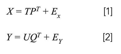
In the formula, T and U mean the score matrices of X and Y. P and Q denote the load matrices of X and Y. EX and EY represent the PLS fitting residual matrices of X and Y. The superscript T denotes the matrix transposition. The linear regression relationship between T and U (U = T * B) can be established from equation [1] and [2]; specifically, B = (TTT)-1TTY. For the prediction of unknown samples, the score matrix Tpre of the spectra array of the samples is calculated first. Then, the concentration is figured out according to the formula Ypre = TpreBQ (22).
The root mean square error of the calibration set (RMSEC) and determination coefficients of the calibration set (R2C) were employed to evaluate the regression model’s fitting effect and stability. The prediction ability of the model was evaluated by the root mean square error of the prediction set (RMSEP), the determination coefficient of the prediction set (R2P), and the ratio of the standard deviation of the prediction set to the standard error of prediction (RPD). The closer the RMSE value is to 0, the better. The closer the R2 value is to 1, and the greater the RPD value is, the better (23). The calculation formulas are expressed as follows:
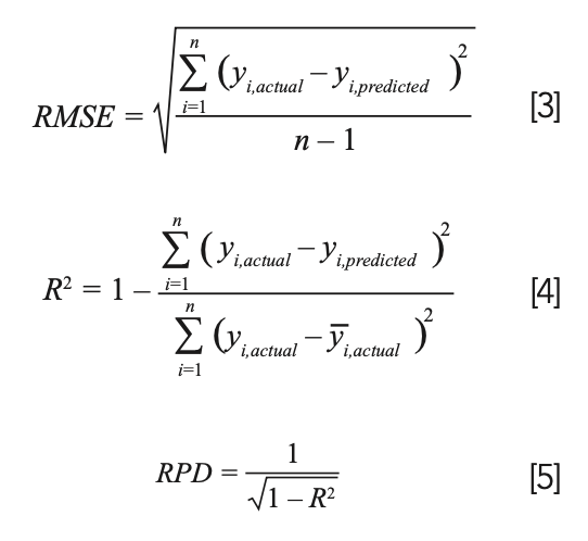
In the formula, n denotes the sample size; yi,actual means the actual measured value of sample i. yi,predicted means the predicted value of sample i based on the regression model.
Outlier Detection
The wrong operation, equipment fault, and environmental disturbance can lead to outliers. Because the outliers are harmful to model performance, it is essential to detect and eliminate the outliers. In this research, the Monte Carlo sampling (MCS) algorithm was used to detect outliers. The basic idea of the MCS algorithm is sample extraction and cross-validation (24), which can be described as follows: first, part of the samples were selected to form a modeling set according to MCS rules. Second, a PLSR model based on the modeling set was established and verified with the remaining samples. Third, the previous two steps were executed circularly to generate the prediction residual array. Fourth, the mean value (MEAN) and standard deviation (STD) for each sample were calculated on the basis of the residual array. Eventually, the outliers were detected intuitively, according to the distribution of MEAN versus STD.
Feature Selection
Throughout the full-range FT-IR spectra, different regions reveal different functional group vibrations. Thus, the mwPLS algorithm was adopted to screen the important regions out according to the following steps. First, a window with a specific width was designed. Then, the window was moved over the entire spectra range from left to right, and the RMSECV at each position where the window arrived was calculated and recorded. Finally, the feature intervals were identified based on the RMSECV values (25).
A bionics algorithm, SFLA, was employed to select feature bands because of its high computing efficiency and excellent global search capability. A Markov chain, which satisfies the steady-state distribution, was simulated in the spectral space to calculate the probability of each band being selected. The characteristic variables are chosen based on the probability values (26). In this research, SFLA and PLSR were utilized comprehensively to select the feature bands from the feature intervals through multiple iterations. The variables were selected according to the absolute value of the PLSR model regression coefficients at each iteration. After all the iterations were run, the probability of being selected for each band can be calculated. The higher the probability, the more important the band is for the model.
Classification
LDA and RF were adopted to classify the samples. The basic idea of LDA is to project the input variable space into the best discriminant vector space to ensure the samples have the largest interclass scatter matrix and the smallest intraclass scatter matrix. The central point of each class was calculated in the projected vector space. For the test samples, the categories were determined by calculating the distance to each center. The shortest one was identified as the category of the test sample (27). The main idea of RF classification was to generate several subsets with significant differences from all samples. Then, each subset was trained to create a decision tree. During the training, a random selected node splitting attribute was introduced. Finally, N decision trees were generated by repeating the above steps. For an unknown sample, the category was determined by all decision trees, and the one with the most votes as the final category was the one used (28).
Hierarchical Clustering
The fuzzy clustering algorithm based on transitive closure was employed to implement the hierarchical clustering of the biofuel pellets. This method mainly includes three steps. First, it starts with normalizing the variable vectors at each dimension to reduce the impact of the differences between different dimensions. Second, it requires constructing a fuzzy similarity matrix and calculating the transitive closure through the self-compositional operation. Third, it continues with performing dynamic clustering according to the λ-truncation matrices inferred from the similarity matrix with different confidence levels (29).
Results and Discussion
Overview of the Spectra
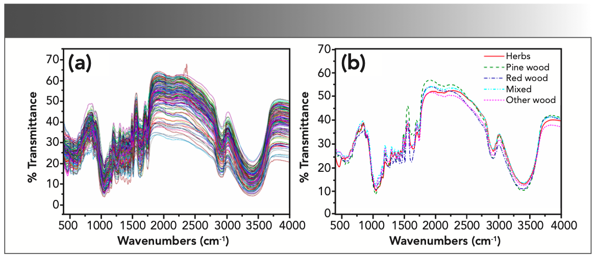
Some elementary points can be observed from the spectra of all the samples (Figure 1a). The spectra of different samples are basically consistent in waveform, whereas the transmittance amplitude shows the gradient variation. It implied that the samples were similar in composition, but the concentrations of the inclusions were different. From the horizontal point of view, it was found that the peak density of different regions was quite varied. The region of 1000–2000 cm-1 has the most abundant peaks. Hence, the fingerprint information most likely locates in this range. In contrast, the tendency of the waveform is relatively smooth in the 2000–2750 cm-1 range. It signifies that the spectral information in this region is probably redundant. The average spectra of the samples manufactured by different raw materials (Figure 1b) show distinct changing tendencies of waveform, which provided the potential feasibility of classification and hierarchical clustering.
FIGURE 1: (a) The transmission spectra of all samples and (b) the average spectra of different categories separated based on raw materials.
Detection and Elimination of Outliers
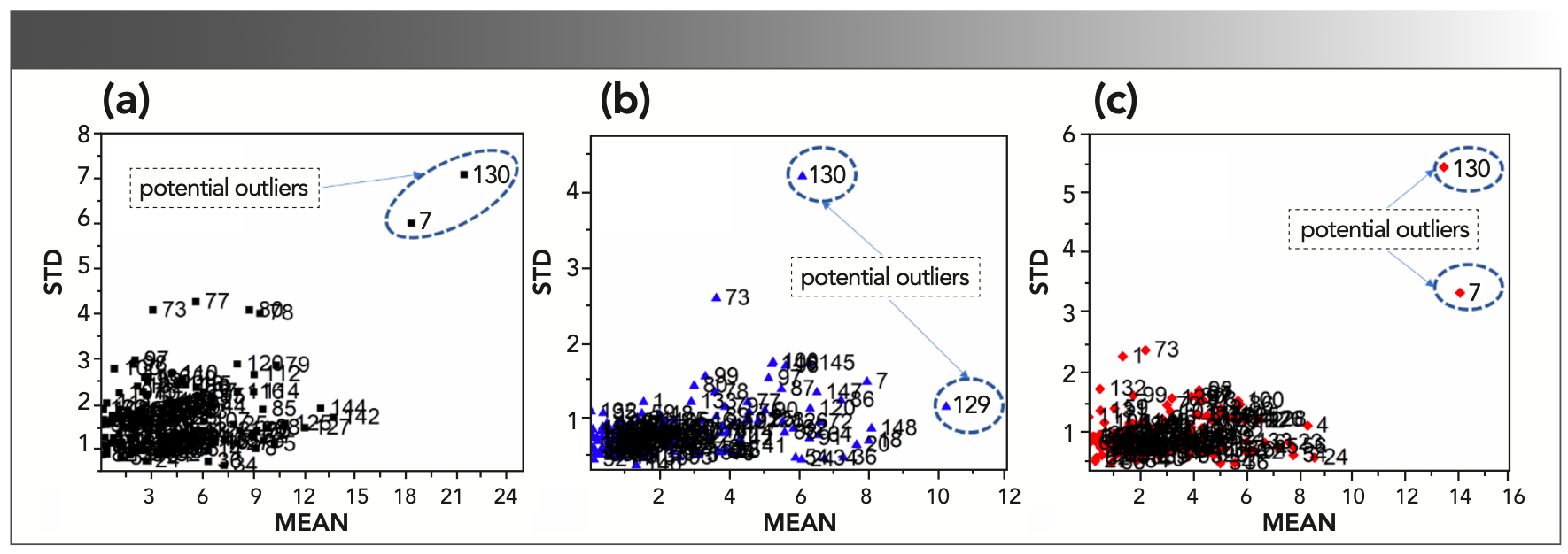
The outliers were detected according to the method mentioned in the section "Outlier Detection." To ensure each sample can be sampled enough times, the iteration times was set to 20,000, and the proportion of the modeling set was set to 0.8. Based on the result obtained after all the loops ending, the scatter plot of MEAN versus STD was generated (Figure 2). According to the dispersion degree, samples 7 and 130 were regarded as potential outliers for cellulose (Figure 2a) and lignin (Figure 2c). Samples 73, 129, and 130 were regarded as potential outliers for hemicellulose (Figure 2b). Through eliminating the potential outliers one by one and evaluating the validation performance, sample 73 of hemicellulose was retained for further analysis because the validation performance became worse when this sample was eliminated.
FIGURE 2: Scatter plots of MEAN versus STD for (a) cellulose, (b) hemicellulose, and (c) lignin.
Preliminary Modeling Analysis
The samples after the outlier elimination were divided into a calibration set and a prediction set for model establishment and external validation. First, the remaining samples were sorted in ascending order according to their chemical concentrations. In the sorted sequence, every four samples with continuous concentration values were treated as a subset. In each subset, the second or the third sample were chosen randomly to constitute the prediction set. As a particular case, the last two samples were treated as a subset, and the first sample was selected into the prediction set. Finally, a calibration set with 110 samples and a prediction set with 36 samples were obtained for each chemical index.
The modeling performance based on the full-range spectra (Table I) proves that there was a strong correlation between the FT-IR spectra and the lignocellulose concentrations. The PLSR models show excellent stability and prediction ability. For cellulose, hemicellulose, and lignin, the R2C values are 0.955, 0.923, and 0.951, and the R2P values are 0.942, 0.878, and 0.868, respectively. By comparing the models for different components, it can be found that the model of cellulose exhibits the best performance. It was mainly caused by the chemical constitution of cellulose, which has less deformation (30).

Feature Intervals Selection
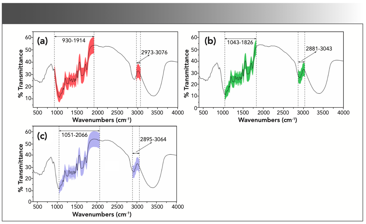
From the view of spectral detection, the lignocellulosic concentration is expressed through the interactions between electromagnetic radiation and various chemical groups. Moreover, the interactions correspond to various wavelength ranges. Therefore, a series of windows with widths from 250 to 500 was designed to slide over the spectra to screen the reasonable feature intervals. For each width, the full cross-validation results were calculated to evaluate the window at each location. Eventually, the feature intervals (Figure 3) were identified by assessing the cross-validation results with different widths (31). For cellulose, the feature intervals were 930–1914 cm-1 and 2973–3076 cm-1 (Figure 3a). For hemicellulose, the feature intervals were 1043–1826 cm-1 and 2881–3043 cm-1 (Figure 3b). For lignin, the feature intervals were 1051–2066 cm-1 and 2895–3064 cm-1 (Figure 3c). It can be found that the intervals 1051–1826 cm-1 and 2973–3043 cm-1 are overlapped for the three components. And the overlapping region occupies a considerable proportion, namely (IntC∩IntH∩IntL)/(IntC∩IntH∩IntL) = 63.56% (the IntC, IntH, and IntL denote feature intervals of cellulose, hemicellulose, and lignin). This observation illustrates that the cellulose, hemicellulose, and lignin are similar in composition but different in specific ingredients, which is consistent with the real situation (32).
FIGURE 3: Feature intervals of (a) cellulose, (b) hemicellulose, and (c) lignin.
The PLSR models’ performance based on the feature intervals (Table II) is slightly better than that based on full-range spectra (Table I). The R2P and R2C values of cellulose, hemicellulose, and lignin are all greater than or equal those in Table I. Hence, the feature intervals selection makes a contribution to reduce the redundant information and improve the model performance.

Feature Bands Selection
To obtain a reasonable assessment for each band, the iteration number of SFLA was set to 50,000; the number of the initial variables was set to 20. According to the importance curve, the thresholds of cellulose (Figure 4b), hemicellulose (Figure 4d), and lignin (Figure 4f) were all set to 0.1. To eliminate the contiguity phenomenon, only the bands at the peak locations were selected as the feature bands. At last, 40, 51, and 84 feature bands were identified for cellulose (Figure 4a), hemicellulose (Figure 4c), and lignin (Figure 4e), respectively.
FIGURE 4: Selection and distribution of feature bands, (a), (c), and (e) are the feature bands of cellulose, hemicellulose, and lignin, respectively; and (b), (d), and (f) are the corresponding selection possibilities of bands calculated using SFLA.
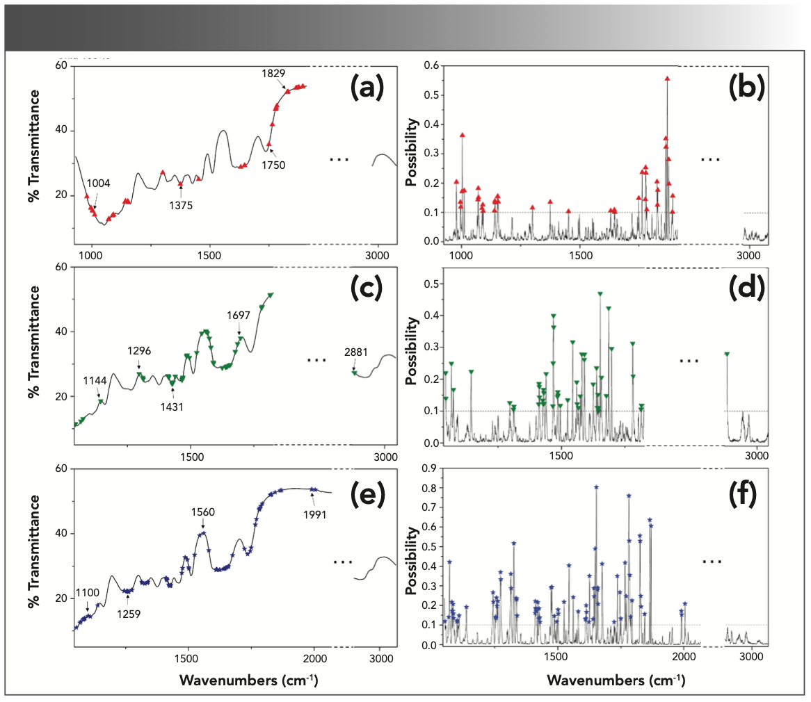
First, the feature bands that were shared by different chemical indexes were counted and analyzed. Six pairs of similar feature bands, 1069, 1141, 1630, 1645, 1783, and 1826 cm-1, shared by the three components were observed. Two pairs of similar feature bands, 1299 and 1452 cm-1, shared by cellulose and hemicellulose indexes were identified. The chemical indexes of cellulose and lignin shared three pairs of similar feature bands: 1750, 1766, and 1865 cm-1. The chemical indexes of hemicellulose and lignin shared ten pairs of similar feature bands: 1043, 1313, 1410, 1424, 1486, 1495, 1524, 1544, 1560, and 1676 cm-1. The assignments of the shared feature bands are summarized below. 1043 cm-1 was assigned to C–O–C asymmetric stretching vi- bration in hemicellulose (33); 1069 cm-1 was assigned to -COO-asymmetrical stretching of aromatic acid in lignin; 1141 cm-1 was assigned to aromatic C-H in-plane deformation typical for guaiacyl propane (34); 1410 cm-1 was assigned to the -COO- stretching vibration in hemicellulose (35); 1424 cm-1 was assigned to the aromatic skeletal vibration or C–H in-plane deformation in lignin and cellulose; 1452 cm-1 was assigned to C-H deformation in -CH3 or C-H bending in -CH2 in lignin and hemicellulose (36); 1630 cm-1 was assigned to C=O stretching vibration in lignin; 1645 cm-1 was assigned to O-H deformation; and 1750 cm-1 was assigned to C=O stretching vibration in ester groups. Then, the exclusive feature bands, which only belong to one chemical index, were counted and analyzed. The exclusive feature bands of cellulose were mainly located at 978–1011 cm-1 and 1374 cm-1. The exclusive bands of hemicellulose were mainly located at 1590, 1685, 1697, and 2881 cm-1. The exclusive bands of lignin were mainly located at 1243–1274, 1467, 1723, 1793, 1845, and 1990 cm-1. The assignments of the exclusive feature bands are summarized below. 1004 cm-1 was assigned to the C–C and C–O stretching vibration; 1243 cm-1 was assigned to the syringyl ring plus C–O stretching in lignin and hemicellulose; 1259 cm-1 was assigned to the guaiacyl ring plus C-O stretching vibration in lignin; 1374 cm-1 was assigned to C-H deformation in cellulose and hemicellulose; 1467 cm-1 was assigned to C-H deformations or asymmetric stretching in-CH3 and -CH2 in lignin; 1590 cm-1 was assigned to aromatic skeletal vibration in lignin; and 2881 cm-1 was assigned to C-H stretching in -CH3 and -CH2 (37).
Based on the above analysis, it can be inferred that the expression of cellulose, hemicellulose, or lignin relied on the synergies of multiple feature bands, which may not make attribution to the actual compounds. Thus, the expression ability of the feature bands to lignocellulose concentrations needs to be verified.
Compared to the PLSR models based on feature intervals (Table II), the PLSR models (Table III) based on the feature bands show better performance in cellulose and lignin, but the model performance of hemicellulose decreases slightly. Beyond that, the redundant information was eliminated effectively under the premise that the model performance remains stable.

Classification
According to the raw materials categories, the samples were divided into “herbs,” “pine wood,” “red wood,” “mixed,” and “other wood.” The “other wood” mainly consists of oak wood, rubber wood, and some tropical wood with fewer parallel samples. To explore the feasibility of bio- fuel pellet classification based on FT-IR spectra, the principal components (PCs) were extracted from the full-range spectra to perform visual analysis. After extraction, the scatter plots based on the first three PCs were generated. It can be found that some points that belong to different categories were overlapped from the oblique upper angle. However, most scatter points of each category were clustered together in the 3D spaces constructed by the first three PCs (Figure 5). Therefore, it is possible to distinguish the categories of samples based on the PCs extracted from the FT-IR spectra.
FIGURE 5: Three-dimensional scatter points based on (a) the first three PCs and (b) broken line of classification accuracy based on different PC numbers.
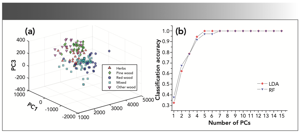
In view of that, the first three PCs don’t exhibit a remarkable ability for the biofuel pellet classification; as a result, more PCs were employed as the input variables to build LDA and RF classifiers. Through validation, it can be found that the classification accuracy of LDA classifier reached 100% when the number of PCs was equal to or greater than four, and the same excellent accuracy of RF was obtained when the number of PCs reached or exceeded eight. The results sufficiently indicate that FT-IR spectra are suitable for the classification of biofuel pellets.
Hierarchical Clustering
The first 15 PCs were introduced as the input variables for hierarchical clustering. Before clustering, the variable vector at each column was normalized by the maximum method to reduce the effect caused by the tremendous value range difference between different PCs. The absolute cosine value between every two samples was calculated to build a fuzzy similarity matrix. After three times self-compositional operations, the transitive closure was obtained. According to the transitive closure, the biofuel pellets could be clustered layer by layer (Figure 6).
FIGURE 6: Dendrogram and heat map of hierarchical clustering.
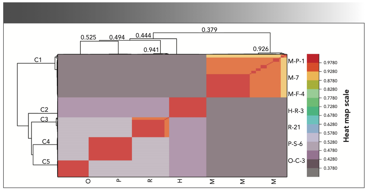
If the confidence level was set to 0.379, the biofuel pellets would be divided into two categories, named “C1” and “OC1.”
If the confidence level was set to 0.444, the “OC1” samples would be subdivided into “C2” and other categories “OC2.”
If the confidence level was set to 0.494, the “OC2” samples would be subdivided into “C3” and other categories “OC3.”
If the confidence level was set to 0.525, all the samples would be clustered into five categories, namely the “OC3” samples were subdivided into “C4” and “C5.”
In addition, the “C1” samples could be subdivided into two categories when the confidence level is greater than 0.926, and the “C3” samples can be subdivided into two categories when the confidence level was set to 0.941.
The hierarchical clustering provides reliable results in the cases of clustering into 2–5 categories. Through referencing the actual categories of the samples, the clustering results “C1,” “C2,” “C3,” “C4,” and “C5” match the “mixed,” “herbs,” “red wood,” “pine wood,” and “other wood” completely.
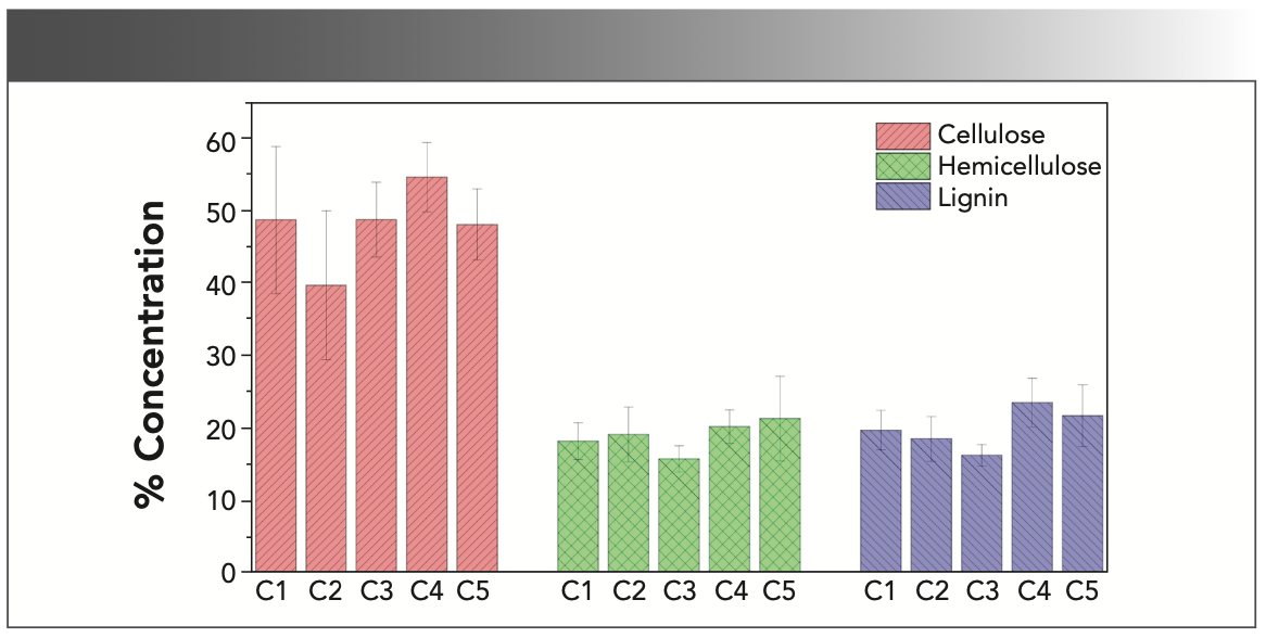
Through the one-way analysis of variance, the cellulose, hemicellulose, and lignin indexes of the samples in Figure 7 all exhibit significant difference between the five clusters with the p values of 7.28e-8, 3.35e-7, and 3.16e-14. Beyond that, multiple comparison analysis was performed to explore the specific relationships between different clusters. For cellulose, the “C2” is significantly different from other categories, the “C4” is significantly different from the “C3” and “C5,” but the difference between the “C3,” “C5,” and “C1” is not significant. For hemicellulose, the “C3” is significantly different from other categories, the “C1” is significantly different from the “C5,” but the difference between the “C2,” “C5,” and “C4” was not significant. For lignin, the “C3” is significantly different from the “C1,” “C4,” and “C5,” the “C1” is significantly different from the “C4,” and the “C4” is significantly different from “C2.” The above analysis illustrates that hierarchical clustering acts in cooperation with the lignocellulose properties of biofuel pellets. Hence, it is convenient for unknown biofuel pellets that pretreatment through clustering the samples with similar properties in to one category.
FIGURE 7: Histogram of concentrations after clustering. Note: In the figure, “C1,” “C2,” “C3,” “C4,” and “C5” represent the clusters obtained by hierarchical clustering; the whisker on the bar indicates the standard deviation.
Conclusion
In this research, a complete scheme for biofuel pellet lignocellulose determination and categorization analysis was designed. Regression models with excellent performance were established to determine the lignocellulose concentration nondestructively. By screening the feature intervals first, the randomness of feature bands extraction was avoided effectively. For categorization analysis, two situations were considered. To distinguish the types of biofuel pellet raw materials, the classifier was built with the utilization of spectral and label information. To estimate the biofuel pellet properties without label information, hierarchical clustering based on transitive closure was performed. Eventually, outstanding results were obtained for classification and clustering. According to the clustering result and the experimental knowledge, the lignocellulose concentration range can be estimated roughly. In a word, it is feasible to determine lignocellulose concentrations, and categorize types and evaluate properties of biofuel pellets based on FT-IR spectra. This research will provide a useful reference to guide the treatments of biofuel pellets.
Frankly speaking, problems still exist in this research. The samples used for analysis were relatively few, which would influence the ability of the model. Hence, more samples should be employed in further studies. The FT-IR spectra were also collected in a laboratory environment, which is not suitable for field detection. Some measures should be taken to improve the practicability of the protocol proposed in this research.
Acknowledgments
Xuping Feng offered us a valuable favor in this paper writing; we would like to express our gratitude to her for the support.
Declarations
Funding
This work has been supported by grants from the National Natural Science Foundation of China (Nos. 61772198, 61772199), Zhejiang Province Public Welfare Technology Application Research Project (No. LGN18F020002), Suzhou Key Industry Technology Innovation Project (No. SYG201808), and the project supported by Key Laboratory of System Control and Information Processing, Ministry of Education, China (No. Scip201804).
Conflicts of Interest and Competing Interests
Liu He, Wenjun Hu, and Yuzhen Wei declare that they have no conflicts of interest.
Availability of Data and Material
Partly available.
Code Availability
Partly available.
Authors’ Contributions
Yuzhen Wei and Liu He contributed to the conception of the study. Liu He performed the experiment. Wenjun Hu and Yuzhen Wei contributed significantly to analysis and manuscript preparation. Yuzhen Wei and Liu He performed the data analyses and wrote the manuscript.
Ethics Approval
This article does not contain any studies with human participants or animals performed by any of the authors.
Consent to Participate
Not applicable.
Consent for Publication
Not applicable.
References
(1) J.J. Wang, and L. Li, Renew. Sust. Energ. Rev. 58, 718–724 (2016).
(2) S.V. Vassilev, C.G. Vassileva, and V.S. Vassilev, Fuel 518, 330–350 (2015).
(3) J. Parobek, et al, BioResources 11(1), 984–995 (2016).
(4) S.S. Su, et al, Int. J. Energy Res. 43(11), 5983–5991 (2019).
(5) V. Tripathi, S.A. Edrisi, and P.C. Abhilash, Renew. Sust. Energ. Rev. 57, 1386–1389 (2016).
(6) Y.Z. Li, et al, Renew. Energy 92, 312–320 (2016).
(7) X.P. Feng, et al, Biotechnol. Biofuels 11, 88 (2018).
(8) X.L. Li, et al, Biotechnol. Biofuels 11, 263 (2018).
(9) S.E. Adebayo, et al, J. Food Eng. 169, 155–164 (2016).
(10) Z.H. You, et al, Appl. Spectrosc. Rev. 50(10), 840–858 (2015).
(11) C.H. Chia, B. Gong, and S.D. Joseph, Vib. Spectrosc. 62, 248–257 (2012).
(12) M. Blanco, J. Cruz, and M. Bautista, Anal. Bioanal. Chem. 392(7–8), 1367–1372 (2008).
(13) D. Cozzolino, Appl. Spectrosc. Rev. 47(7), 518–530 (2012).
(14) M. Allard, M. Piche, and F. Babin, Appl. Optics. 54(10), 2594–2605 (2015).
(15) W.N. Liu, et al, Bioresour. Technol. 124, 306–310 (2012).
(16) T.J. Kinney, et al, Biomass Bioenerg. 41, 34–43 (2012).
(17) S. Nanda, et al, Biomass Bioenerg. 91, 56–68 (2016).
(18) R.M. Balabin,and S.V. Smirnov, Anal. Chimica Acta. 692(1–2), 63–72 (2011).
(19) R. Priya, J.F.P. Dass, and R. Siva, Plant Mol. Biol. Rep. 34(3), 618–627 (2016).
(20) P.J.V. Soest, Federation Proceedings 32(7), 1804 (1973).
(21) I.S. Helland, et al, J. Chemometr. 32(9), e3044 (2018).
(22) R. Romano, et al, J. Chemometr. 33(3), e3105 (2019).
(23) M.C. Korkmaz, et al, J. Stat. Manag. Syst. 22(5), 871–891 (2019).
(24) W.S. Cai, D. Chen, and X.G. Shao, Vib. Spectrosc. 47(2), 113–118 (2008).
(25) S.H. Wang, et al, Anal. Chim. Acta. 1000, 109–122 (2018).
(26) X. Li, et al, Inf. Sci. 192, 143–151 (2012).
(27) L.R. Costa, P.F. Trugilho, and P.R.G. Hein, Biomass Bioenerg. 112, 85–92 (2018).
(28) S.F. Li, M.Z. Jia, and D.M. Dong, Spectrosc. Spect. Anal. 38(6), 1766–1771 (2018).
(29) H.S. Lee, Fuzzy Sets Syst. 123(1), 129–136 (2001).
(30) Y.L. Song, et al, Bioresour. Technol. 193, 164–170 (2015).
(31) Y. Gu, et al, J. Biomed. Opt. 21(1), 015002 (2016).
(32) H. Kawamoto, T. Hosoya, and S. Saka, J. Anal. Appl. Pyrolysis 80(1), 118–125 (2007).
(33) C. Cao, et al, Cellulose 22(1),139–149 (2015).
(34) J.B. Chen, S.Q. Sun, and Q. Zhou, Anal. Bioanal. Chem. 405(29), 9385–9400 (2013).
(35) X.Q. Wang, and H.Q. Ren, J. Wood Sci. 55(1), 47–52 (2009).
(36) E.D. Tomak, et al, Int. Biodeterior. Biodegrad. 85, 131–138 (2013).
(37) X.Y. Zhang, et al, Int. Biodeterior. Biodegrad. 60(3), 159–164 (2007).
Liu He, Wenjun Hu, and Yuzhen Wei are with the School of Information Engineering at Huzhou University, in Huzhou, China, and with the Zhejiang Province Key Laboratory of Smart Management Application Agricultural Resources at Huzhou University, in Huzhou, China. Direct correspondence to Yuzhen Wei at: doctorwhy08@163.com ●

AI Shakes Up Spectroscopy as New Tools Reveal the Secret Life of Molecules
April 14th 2025A leading-edge review led by researchers at Oak Ridge National Laboratory and MIT explores how artificial intelligence is revolutionizing the study of molecular vibrations and phonon dynamics. From infrared and Raman spectroscopy to neutron and X-ray scattering, AI is transforming how scientists interpret vibrational spectra and predict material behaviors.
Real-Time Battery Health Tracking Using Fiber-Optic Sensors
April 9th 2025A new study by researchers from Palo Alto Research Center (PARC, a Xerox Company) and LG Chem Power presents a novel method for real-time battery monitoring using embedded fiber-optic sensors. This approach enhances state-of-charge (SOC) and state-of-health (SOH) estimations, potentially improving the efficiency and lifespan of lithium-ion batteries in electric vehicles (xEVs).
New Study Provides Insights into Chiral Smectic Phases
March 31st 2025Researchers from the Institute of Nuclear Physics Polish Academy of Sciences have unveiled new insights into the molecular arrangement of the 7HH6 compound’s smectic phases using X-ray diffraction (XRD) and infrared (IR) spectroscopy.