Simulation of an Algorithm for Space Target Materials Identification Based on vis-NIR Hyperspectral Data

Space target recognition is of great importance for maintaining aerospace safety and national security. When observing a space target, owing to the low spatial resolution of ground-based observation equipment, each pixel in a hyperspectral image might represent a mixture of several different materials. Hyperspectral unmixing is a process used to extract the endmembers and their corresponding abundances from hyperspectral data. Unfortunately, most existing methods cannot make full use of the available spatial information data. The paper proposes a new local manifold sparse regularized unmixing model based on similarity regularized nonnegative matrix factorization (SRNMF). To exploit the spatial information of the vis-NIR (approximately 400–2500 nm) hyperspectral image of a space target, image segmentation is introduced to generate similar local regions. These local regions are generated adaptively, and pixels within each region have similar abundance sparseness. Simulation experiments validated the high efficiency and precision of the proposed algorithm, which should also be suitable for other spectral analysis applications.

A space target in the aerospace field usually refers to a man-made spacecraft or item of space debris orbiting the earth outside the limit of the atmosphere (1). With the rapid development of modern science and technology, increasing numbers of satellites are being sent into space, and Earth’s orbital space is becoming increasingly crowded. Therefore, the study of space objects is becoming of greater importance.

Owing to the spatial distance limitation, a ground-based observer cannot identify a space target through direct observation of local information. However, differences in the reflection spectra of the various materials comprising the surface composition of a space target provide unique spectral information that allows identification of space targets (2). Spectral analysis can be used to analyze the composition of space objects and the proportions of the different constituent space materials, allowing identification of space targets. With the rapid development of satellite and remote sensing technology, hyperspectral imaging has received increased attention because its numerous spectral bands can provide greater information for spectral analysis (3). However, owing to spatial resolution limitations, mixed pixels are commonly found in hyperspectral images, the existence of which can markedly affect the results of spectral analysis. Therefore, the goal of hyperspectral unmixing is to decompose mixed pixels into the constituent materials, called endmembers, and to determine their corresponding fractional abundances (4,5). Most existing hyperspectral separation methods are based on linear mixed models that assume mixed pixels are linear combinations of endmembers. In general, conventional algorithms for hyperspectral unmixing involve two steps—endmember extraction and mixed-pixel decomposition. Common endmember extraction algorithms include vertex component analysis (VCA). After endmember extraction, relevant abundance maps are usually obtained using fully constrained least squares (FCLS) analysis.

Nonnegative matrix factorization (NMF) is a statistical method typically used for hyperspectral unmixing. The NMF approach decomposes a data matrix into two low-rank matrices with nonnegative constraints. However, it should be noted that standard NMF methods might not guarantee solution uniqueness; thus, the decomposition result usually depends on the initialization (6). Constraints on endmembers and abundances have been exploited and used in NMF applications. Minimum volume constrained NMF (MVCNMF) (7) exploits the convex geometry information of mixed pixels and adds a volume constraint to NMF. In the case of low signal noise, although the performance of the MVCNMF algorithm is superior, MVCNMF cannot handle large data sets because of the large amount of computational overhead. Recently, owing to the sparse distribution of spatial materials, sparse constraints have been added to NMF to generate unique solutions that lead to improved results, such as L1 sparsity NMF (8) and L1/2 sparsity NMF (9).

In this paper, the SRNMF unmixing model is proposed, incorporating a spatial group sparsity regularizer and a sparse measure function regularizer into an NMF-based unmixing process. Thus, the SRNMF is able to explore the spatial information and the sparse structure of hyperspectral images. In addition, because of the high similarity between neighboring pixels in the hyperspectral data, simple linear hierarchical clustering (SLIC) is used to describe the similarity. The SLIC can obtain a number of meaningful homogeneous regions of the spectra that are spatially adjacent to each other. The paper considers the sparse spatial distribution of the target material and the spatial information, and introduces sparse regularizers to represent the spatial information. Integration of both the spatial structure information and the sparse properties means SRNMF can obtain improved unmixing results in comparison with other popular unmixing algorithms.

Related Work

A Linear Mixed Model

The linear mixed model, as a straightforward and efficient way to represent mixed pixels, assumes that the spectral response of a pixel is a linear combination of all the pure spectral signatures (endmembers) present in the pixel (10). Mathematically, if we let Y = [y₁, y₂...y_N] ε Ʀ^L×^N denote a hyperspectral data matrix that consists of N pixels with L bands, then the linear mixed model for each pixel can be written as follows:

where M is the number of endmember signatures in the scene, y_j = [y_1j, y_2j...y_Lj] ^T ε Ʀ^L is the measured value of the reflectance at spectral band j, s_j = [s_1j, s_2j...s_Mj] ε Ʀ^M is the abundance vector of y_j, and εj represents the error term for spectral band i.

As each pixel in a scene is assumed to share the same set of endmembers A, the hyperspectral data Y comprising N pixels can be written as follows:

where N represents the noise matrix, S represents the fractional abundances of the endmembers in the scene, and A is an L × M matrix containing M endmembers. Additionally, according to the definition of “abundance,” all abundance values should be nonnegative, and the summation of the abundance values for one pixel must equal one. Therefore, the following two physical constraints must be fulfilled: abundance sum-to-one constraint (ASC) ∑_j S_jn = 1 and abundance nonnegative constraint (ANC) S_jn >0 (11).

Nonnegative Matrix Factorization

NMF decomposes a set of highly dimensional data into two nonnegative matrices, and it finds “basis vectors” by which the original data are approximated through linear combination (12,13). Additionally, NMF can satisfy the nonnegative requirements of both the endmember matrix and the abundance matrix of hyperspectral data, and its representation is similar to that of hybrid pixel decomposition based on the spectral linear mixed model. Moreover, it has good anti-noise performance, and so it is used widely in hyperspectral unmixing applications.

Given the observation matrix Y = [y₁, y₂...y_N] ε Ʀ^L×^N, the objective of NMF is to determine two matrices: A ε Ʀ^L×^M and S ε Ʀ^M×^N, in which all elements are nonnegative and Y ≈AS holds true, where M is a positive number (M < min[L,N]).

To solve the problem, the paper defines cost functions constructed to quantify the quality of the approximation, which leads to the following optimization problem:

where ǁ·ǁ_F is the Frobenius norm defined as ǁYǁ_F = (∑_ij |y_ij|²)^1/2, and all elements in A and S are unknown and nonnegative. Although equation 3 is convex with respect to both A and S separately, it is nonconvex for both variables in combination (14). The gradient-based alternating nonnegative least squares (ANLS) method (14,15) was used to solve the above problem; when one of the matrices was updated, the other remains fixed. The computation breaks down the optimization problem into two subproblems:

where the positive parameters α_k and β_k are step sizes. The gradient used at each sub-iteration can be calculated as follows (16):

The gradient descent method first finds the gradient, selects the appropriate step size, and finds the optimal solution in a step-by-step process along the direction of the gradient descent; it also uses the negative gradient direction as the search direction. The closer to the target value, the smaller the iterative step size and the slower the forward speed. Therefore, the most important stage in the method is the selection of the iterative step size. The gradient descent method does not find an exact optimal solution after a finite number of iterations, but it will infinitely approach the optimal solution at a slower speed.

Proposed NMF with Sparse Constraints for Hyperspectral Unmixing

As mentioned above, an NMF-based hyperspectral unmixing algorithm automatically estimates the number of endmembers and their relative abundances. Moreover, it is applicable to situations where there is little prior information in the scene. However, it fails to take into consideration the sparse prior information on abundances and manifold structures hidden within hyperspectral data, which are essential for the hyperspectral unmixing problem. Owing to the spatial autocorrelation property of space target material distribution, the inclusion of spatial information into the spectral unmixing process can improve the accuracy of both endmember extraction and abundance estimation. Here, the paper considers the sparse spatial distribution of the target material and spatial information, introduces sparse regularizers to represent the spatial information, and describes the process of unmixing mixed pixels of space targets.

To integrate the sparse prior information on abundance and spatial structure into the hyperspectral unmixing process, the SLIC (17) image segmentation algorithm can be used to divide a hyperspectral image into different spatial groups. SLIC is an adaptive k-means super-pixel generation method, which is simple in structure, fast in operation, and contains few parameters. Here, an improved SLIC algorithm is put forward as part of the hyperspectral unmixing process.

The main steps of the process are as follows.

(1) Initialize the cluster center and distribute the seed points evenly within the image, according to the set number of super-pixels.

(2) Reselect the seed point in the neighborhood corresponding to the seed point. Calculate the gradient value of all seed points in the neighborhood, and set the minimum gradient value as the new seed point. This process helps avoid the seed point falling on the contour boundary of the gradient, which affects the subsequent clustering effect. The paper introduces a regular hexagonal grid to select the corresponding neighborhood (18).

(3) In the region of 2w × 2w, calculate the distance from the pixel to the seed point; for example, the cluster center, where w is the desired super-pixel size (that is, the width of the regular hexagon). Then, perform the generation using the k-mean algorithm until the algorithm converges or reaches a set number of iterations. It should be noted that the original spectral characteristics are used directly in the clustering process, minimizing the loss of spectral information. For hyperspectral images with L bands, the cluster center of the i-th super-pixel is defined as follows:

where xⁱ = [x_1i, ..., x_Li]^T is the mean spectral reflectance of the i-th super-pixel, and [mⁱ, nⁱ]^T represents the spatial coordinates of the i-th cluster center. The distance calculation formula is as follows:

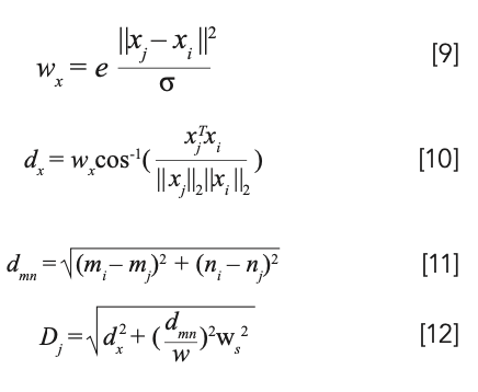
where d_x denotes the spectral distance, d_mn denotes the spatial distance, w_x is the weight of the spectral similarity measure (x_j is the distance weight to the cluster center; the closer to the center cell location, the greater the weight), D_j computes the distance between pixel x_j and the cluster center (which is normalized according to the width of the hexagon w), and w_s can be 0.3, which denotes the importance of spectral similarity and spatial similarity. Here, w controls the average size of the super-pixels and the total number of space groups P. In this paper, w was considered as 5.

(4) Merge outliers. The area of the connected component is judged according to the 4-neighbor or 8-neighbor connection; if the area is too small, it is classified into the nearest label.

As the hyperspectral image is cut into different space groups, the paper introduces the sparse regularity of the combined space group structure based on the sparse NMF. For a given set of hyperspectral data Y_r = [Y^I,...,Y^P] ε Ʀ^L×^N, where P is the number of super-pixels and the submatrix Y^P ε Ʀ^L×^n_p, the abundance matrix is divided into P groups as S_r =(S¹,...,S^P) ε Ʀ^M×^N. Owing to the spatial structure characteristics, each space group has the same endmembers, corresponding to a similar abundance matrix. Therefore, the final objective function is as follows:

where function

is a measurement of sparseness (19), m denotes the number of endmembers, λ and β denote the regularization terms that weight the reconstruction error and the space group sparseness and the abundance, respectively, S^P = [s₁,...s_np] ε Ʀ^M×^np denotes the abundance matrix of spatial group

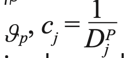
denotes the degree of local similarity between pixels and cluster center pixels, s^P = [s^P[1],..., s^P[M]]^T is the average abundance sparseness constraint (that is, groups for which the corresponding abundance matrix structure is similar), and m is the number of endmembers.

The corresponding endmember and abundance values are solved by block coordinate descent, which can approximate the objective function for one variable block at a time, while the other variable blocks remain unchanged. For the proposed objective function (equation 13), the optimization consists of three main subproblems in the iteration: (1) updating s^P; (2) updating the abundance matrix S^P; and (3) updating the endmember matrix A. Then, each subquestion is solved using the ANLS algorithm, for which the update rules for each abundance group S^P and endmember matrix A are introduced as follows:

The ASC should be added in the learning of the abundances. Therefore, the paper introduces an effective method used in FCLS (20), where the endmember matrix A and each spatial group Y^P are augmented before the learning of the abundance matrix, for example:

where δ is a positive value used to balance the estimate accuracy and additivity constraint.

As the endmember matrix A changes, s^P changes in each step of the generation. For each of p = 1, 2, ..., P, s^P can be calculated as follows:

where y^p is the mean spectral vector of the p-th super-pixel, s^P = [s^P[1],..., s^P[M]]^T is the average abundance vector, and

According to the multiplication update rule, the following formula can be obtained:

As the endmember matrix has no constraints, the gradient of A is easy to solve. The update rules for the endmembers are as follows:

and the abundance update rules are as follows:

Based on the above derivation, we can obtain the final update rule as follows:

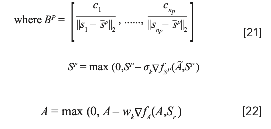
where w_k = w₀ β^tk, β ε (0,1), step size is selected based on the Armijo rule (21), and t_k is the first nonnegative integer t that satisfies the sufficient decreasing condition.

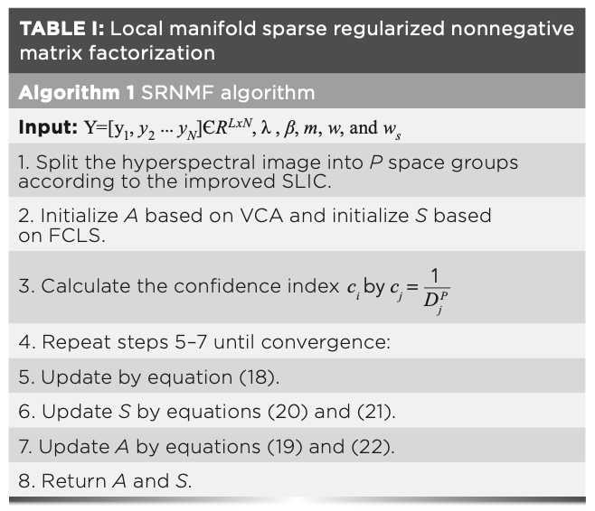
The procedure of the proposed SRNMF is described in Table I.

Experiments

The paper designed a series of experiments to evaluate the performance of the proposed SRNMF algorithm. Both MVCNMF and VCA-FCLS are used for comparison with the proposed method. To evaluate the unmixing results, the following two performance metrics were adopted: the spectral angle distance (SAD) and the root mean square error (RMSE). The SAD, which is used to evaluate the performance of endmember estimation, is the angle distance between an estimated endmember and its corresponding truth. The SAD for the p-th endmember is defined as follows (22):

where Â_p is the corresponding estimated result, and A_p denotes the truth of one endmember. The smaller the SAD value, the closer the extracted endmember spectrum is to the real spectrum.

The RMSE, which is used to evaluate the performance between the estimated abundance S_p and the corresponding truth Ŝ_p, is given by the following (23):

where N is the number of pixels in the hyperspectral image, and smaller values of the RMSE correspond to better performance.

The volume of data in a real hyperspectral image is large, and the calculation is time-consuming. Characteristics of endmember types are complex and variable, and specific information of abundance is unknown. However, a synthetic analog hyperspectral image has only a small amount of data, and rapid calculation speed; furthermore, both the endmember numbers and their abundances are known. Therefore, the performance of the proposed algorithm was assessed based on tests using synthesized analog image data.

Simulated Data Set 1

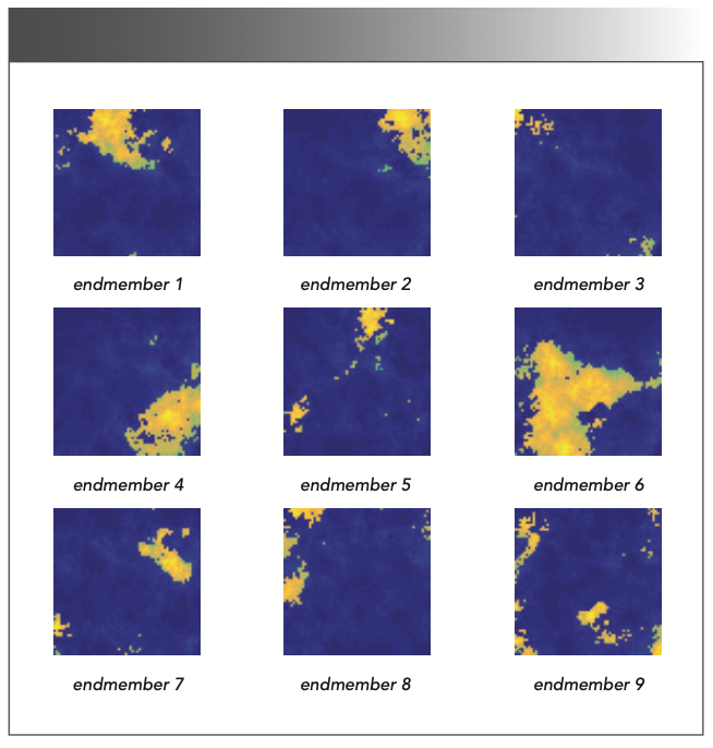
To be representative for evaluation, the synthetic data should have characteristics similar to a real hyperspectral image, and the generation of abundances should conform to the characteristics of real images, such as in terms of local dominance and distinct contour. To generate the synthetic data, the paper selected some true mineral spectra from the U.S. Geological Survey digital spectral library, while the corresponding abundance maps were generated in accordance with a spherical Gaussian field. The data were generated using a linear mixed model with M randomly selected signatures as endmembers and with ASC imposed in each simulated pixel. In this experiment, M was varied from 5–11, with an interval of 2. The first simulated data set (DC1), which comprised 224 spectral channels and 64 × 64 pixels, was generated using the Hyperspectral Imagery Synthesis toolbox in Matlab (http://www.ehu.es/ccwintco/index.php/Hyperspectral_Imagery_Synthesis_tools_ for_MATLAB). This allows the user to choose appropriate parameters for the simulation procedure, such as the spatial dimensions, distribution of abundances, and number of endmembers M, which provides the user considerable flexibility and choice. A synthetic image was produced without the existence of pure pixels. The ground-truth abundance maps of DC1 for the case with nine endmembers are shown in Figure 1. To evaluate the performance of resistance to noise, zero-mean white Gaussian noise was added to the synthetic data.

FIGURE 1: Abundance maps of the simulated data set 1 when endmember number is 9.

Simulated Data Set 2

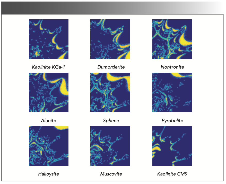
A second set of simulated data (DC2) was built comprising 221 spectral channels and 100 × 100 pixels. It used nine endmembers selected from the U.S. Geological Survey spectral library. Figure 2 shows the spectral and Figure 3 shows the abundance maps for the nine endmembers: kaolinite KGa-1, dumortierite, nontronite, alunite, sphene, pyrobelite, halloysite, muscovite, and kaolinite CM9. Under nonnegative and additive constraints, k-means clustering (24) and Gaussian filtering were used to generate the corresponding abundance maps. The generation process adopted was same as that of Hendrix and associates (25), which can be described as follows:

(1) use the fractal method to create a 100 × 100 hyperspectral scene

(2) divide the generated scene into several clusters using the k-means algorithm

(3) assign a spectrum signature to each cluster according to the rules.

(4) Ultimately, the DC2 data set had the following characteristics;

(5) The simulated image did not contain completely pure pixels, and all the simulated pixels in an area were mixed.

(6) Pixels near the edge of an area were more mixed than pixels at the center of the area.

(7) If the simulation area was sufficiently large, the pixel at the center could exhibit final purity of 99% of the final members. After generating DC2, the scene was again contaminated with both white and correlated noise.

FIGURE 2: Spectra of nine endmembers for the simulated data set 2 (kaolinite KGa-1, dumortierite, nontronite, alunite, sphene, pyrobelite, halloysite, muscovite, and kaolinite CM9).

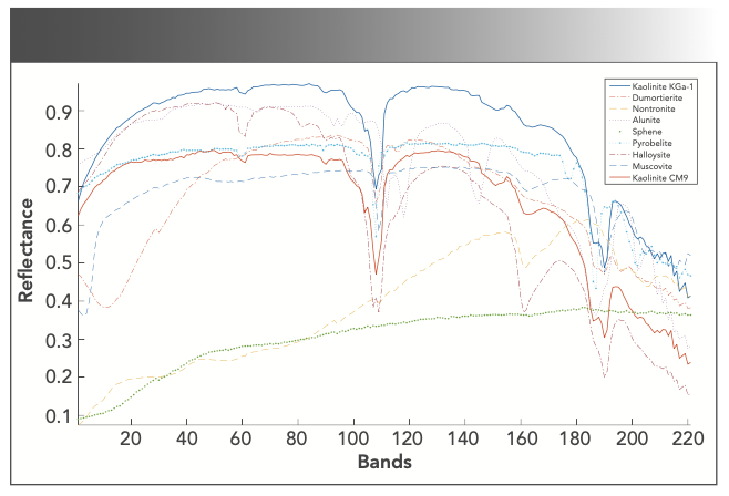
FIGURE 3: Abundance maps of nine endmembers for the Simulated Data Set 2 (kaolinite KGa-1, dumortierite, nontronite, alunite, sphene, pyrobelite, halloysite, muscovite, and kaolinite CM9).

All experimental results analyzed in this paper are the averages of 20 randomized trials. This paper used VCA-FCLS as the default initialization for all the NMF-based methods. In addition, the tunable parameters of the comparison algorithm were consistent with the original reference.

Experiment 1

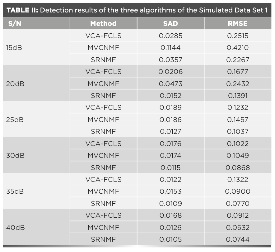
In Experiment 1, the DC2 data set was polluted with Gaussian white noise and Poisson noise with different noise levels, where the signal-to-noise ratio (S/N) was varied from 15–40 dB with an interval of 5 dB, and where the relevant parameters were assigned as follows: w = 5, m = 9, w_s = 0.5, λ = 0.3, and β = 0.2. The number of endmembers was known in advance for all the algorithms.

It can be seen from Table II that the proposed SRNMF compared favorably with the other algorithms in terms of the SAD and RMSE values in most S/N cases. All the tested algorithms obtained RMSE values lower than the abundance of 0.5 and the endmember angle errors were all <0.2. Meanwhile, all algorithms showed a decrease in unmixing accuracy as the signal-to-noise ratio (S/N) decreased. For a value of S/N ≤ 35 dB, the spectral element error and abundance RMSE corresponding to the SRNMF algorithm were found superior to the other algorithms.

Experiment 2

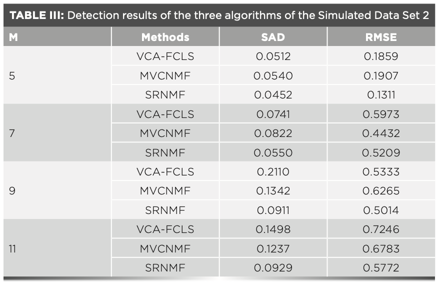
In a hyperspectral image scene of the actual space target, the number of endmembers is complex and variable, and the number of different endmembers might have some uncertain effects on the algorithm. The paper conducted experiment 2 using the DC1 data set to verify the applicability of the proposed method with regard to different numbers of endmembers. This experiment was conducted under the condition of 20 dB Gaussian white noise, and the number of endmembers M was varied from 5 to 11.

As shown in Table III, the performance generally decreased as the number of endmembers increased. For a relatively small value of M, the overall unmixing precision of all tested algorithms was similar; however, the SRNMF algorithm was clearly superior as the value of M increased.

Conclusions

This paper proposed an improved local manifold SRNMF algorithm for pixel unmixing in relation to space targets. The proposed SRNMF algorithm does not require a pure pixel hypothesis, makes full use of the internal structural information of hyperspectral data, and is more robust than other algorithms to the effects of noise. An improved SLIC segmentation method can divide hyperspectral images into different local homogeneous regions. In addition, the local sparse structure of combined spatial information can describe the local distribution of the endmembers of space targets. Experimental results obtained using simulated data confirmed the potential of the proposed algorithm. Moreover, the method could provide accurate results for spectral unmixing in cases with little prior information and low S/N ratios. The proposed algorithm has wide-ranging prospects in the field of space object recognition.

Funding

This work was supported by the National Natural Science Foundation of China under Grant [No. 61575015].

Disclosures

The authors declare that they have no conflict of interest.

References

(1) H. Xiao, Satellite & Network 11, 64–70 (2017).

(2) D. Bédard and M. Lévesque, J. Spacecr. Rockets 51, 1492–1504 (2014).

(3) J. Liu, Z. Tang, Y. Cui, and G. Wu, Sensors 17, 1364–1391 (2017).

(4) F. Zhu, Y. Wang, S. Xiang, B. Fan, and C. Pan, ISPRS J. Photog. Remote Sens. 88, 101–118 (2014).

(5) J.M. Bioucas-Dias, A. Plaza, N. Dobigeon, M. Parente, Q. Du, P. Gader, and J. Chanussot, IEEE J. Sel. Topics App. Earth Observ. Remote Sens. 5, 354–379 (2012).

(6) D.D. Lee and H.S. Seung, Nature 401, 788–791 (1999).

(7) L. Miao and H. Qi, IEEE Trans. Geosci. Remote Sens. 45, 765–777 (2007).

(8) Y. Yuan, M. Fu, and X. Lu, IEEE Trans. Geosci. Remote Sens. 53, 2975–2986 (2015).

(9) R. Huang, X.Li, and L. Zhao, Remote Sens. 9, 1074 (2017).

(10) N. Keshava, Lincoln Laboratory Journal 14, 55–78 (2003).

(11) D. Heinz and C.I. Chang, IEEE Trans. Geosci. Remote Sens. 39, 529–545 (2001).

(12) S.A. Vavasis, SIAM J. Optim. 20, 1364–1377 (2009).

(13) X. Liu, W. Xia, B. Wang, and L. Zhang, IEEE Trans. Geosci. Remote Sens. 49, 757–772 (2011).

(14) T. Hastie, R. Tibshirani, J. Friedman, and J. Franklin, Math. Intell. 27, 83–85 (2005).

(15) C.J. Lin, Neural Comput. 19, 2756–2779 (2007).

(16) C. Févotte, N. Bertin, and J.L. Durrieu, Neural Comput. 21, 793–830 (2009).

(17) R. Achanta, A. Shaji, K.Smith, A. Lucchi, P. Fua, and S. Süsstrunk, IEEE Transactions on Pattern Analysis and Machine Intelligence 34, 2274–2282 (2012).

(18) E. Luczak and A. Rosenfeld, IEEE Trans. Comput. 25, 532–533 (1976).

(19) Y. Qian, S. Jia, J. Zhou, and A. Robles-Kelly, IEEE Transactions on Geoscience and Remote Sensing 49, 4282–4297 (2011).

(20) D.C. Heinz, IEEE Trans. Geosci. Remote Sens. 39, 529–545 (2001).

(21) D.P. Bertsekas and J. Opera, Research Soc. 48, 334–334 (1997).

(22) N. Keshava and J.F. Mustard, IEEE Signal Process. Mag. 19, 44–57 (2002).

(23) A. Plaza, P. Martinez, R. Perez, and J. Plaza, IEEE Trans. Geosci. Remote Sens. 42, 650–663 (2004).

(24) J.A. Hartigan and M.A. Wong, J. Royal Statistical Soc. 28, 100–108 (1979).

(25) E.M.T. Hendrix, I. Garcia, J. Plaza, G. Martin, and A. Plaza, IEEE Trans. Geosci. Remote Sens. 50, 2744–2757 (2011).

Qingbo Li, Ruiguang Zhao, and Xingjin Miao are with the School of Instrumentation and Optoelectronic Engineering and the Precision Opto-Mechatronics Technology Key Laboratory of Education Ministry at Beihang University, in Beijing, China. Direct correspondence to Qingbo Li at qbleebuaa@buaa.edu.cn ●