More About CLS, Part 2: Spectral Results (Not Needing Constituent Values) and CLS

In our previous column, we introduced a set of data suitable for more extensive examination than was permitted in our previous discussion of the classical least squares (CLS) algorithm. In this column, we start to analyze the data using two methods (CLS and principal component analysis [PCA]) that do not involve the concentrations of the components of the mixtures. We begin our expansion of the analysis by examining the data from the 70-sample data set the same way we did for the previous 15-sample data set. First, we examine the spectral results, and then apply the CLS algorithm to verify the previous findings. Neither of these types of analysis requires the use of external constituent information. We then further expand the analysis by calculating principal components. 

Although the goal of this column is to examine the effects of using volume fractions vs. weight fractions as the constituent concentrations for principal component regression (PCR) and partial least squares (PLS) calibrations, there is much to be learned from the spectroscopic data itself, without reference to any constituent compositions. Therefore, our initial inspection of the data parallels the initial examination of the smaller, 15-sample set of mixtures, to verify that those computed values did not require concentration values, or involve the application of advanced chemometric calibration algorithms. Instead, our initial foray into looking at the results from the statistical experimental design described in the previous column (1) was to examine the behavior of the spectral data alone, without involving the use of chemometrics. The application of chemometrics to the data will be described later, and for reasons that will become clear, may not be described fully here. The advantage of analyzing the spectral data without bringing in the constituent values is that the expectations of their behavior are better known, and more easily described. This allows us to compare our results with the theoretical expectations, so that when we introduce the constituent values, we will have some foreknowledge of how we might expect the data to behave. Some of these behaviors have already been listed qualitatively in Tables I and II (see the previous column [1]), where we compared current near-infrared (NIR) spectroscopy practice to theoretical expectations.

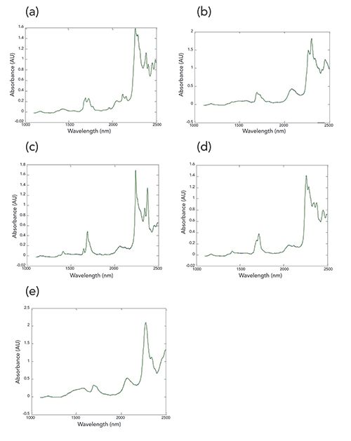
While we have spectra of the pure materials that comprise the mixtures, they were not taken as part of the calibration set. Therefore, for comparison and demonstration purposes, we use the five mixtures containing each of those materials at 60% (the maximum value they can attain in these samples) with each of the other mixture components at their lowest value (10%) as surrogates for the pure materials. The plots in Figure 1 present these spectra, for reference.

Figure 1: Spectra of selected mixtures. Each of the spectra represents one of the mixtures, which contains the maximum concentration (60%) of the component corresponding to the label for that spectrum: (a) acetone, (b) butanol, (c) dichloromethane, (d) dichloropropane, and (e) methanol. Each of the other four components present in that mixture are at their minimum concentrations (10%). The pair of measured spectra from each mixture are plotted on the same axes; it is clear that all these pairs of spectra exactly overlap, showing only the second plotted spectrum in each case.

CLS Results

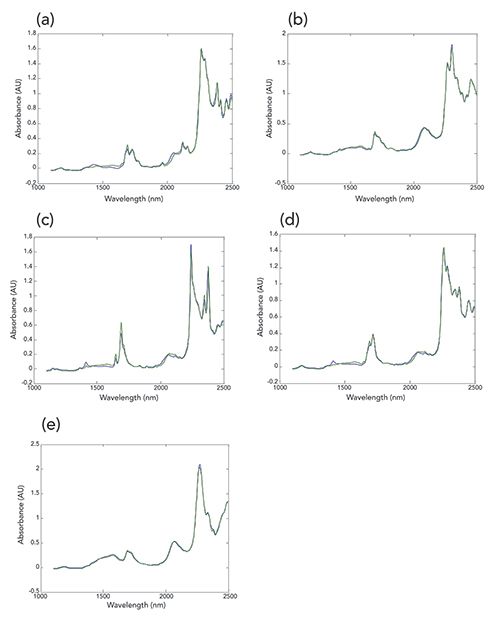
In keeping with our desire for initial analysis to not use the reference values, our next activity is to present the results of performing classical least squares (CLS) analysis on the mixture data. One aspect of CLS gives us the ability to reconstruct the spectrum of a sample from the spectra of the pure components. Thus the validity of the data analysis, as well as the quality of the data, can be captured by CLS analysis by the agreement between a pure-component spectrum computed from the mixture spectra and the measured spectrum of that chemical component. These plots are shown in Figure 2, for the mixtures containing the maximum amount (60 wt%) of each of the ingredients respectively, and for each mixture the minimum amount (10 wt%) of all the other ingredients. It is clear that the agreement between the theoretical reconstructed spectrum and the actual spectrum of each ingredient is almost, although not quite, as good as the agreement between duplicate spectra of the same material. This an important observation, since later on we will be comparing spectra to each other, and knowing the amount of deviation expected between actual measurements and computed approximations will be important in evaluating the computed results.

Figure 2: Comparisons between the actual measured spectra of the five mixtures containing the maximum amount (60 wt%) of each mixture component, and the reconstruction of that spectrum using the CLS algorithm. In all cases. blue = measured spectrum, green = reconstructed spectrum using CLS algorithm. Spectra shown include: (a) acetone, (b) butanol, (c) dichloromethane, (d) dichloropropane, and (e) methanol.

In Figure 3, we have plotted, for each of the five ingredients, the values of the CLS-calculated concentrations vs. the known weight percent and volume percent of the ingredients. Not surprisingly, we note the following characteristics of the plots in Figure 3:

Figure 3: Spectrally calculated values versus reference weight fraction and volume fraction, for the five components in the mixtures. In all plots, the ordinate is the spectrally calculated value, and the abscissa is the weight or volume fraction value, as marked. Figure plots are for the following compounds: (a,b) acetone, (c,d) butanol, (e,f) dichloromethane, (g,h) dichloropropane, and (i,j) methanol.

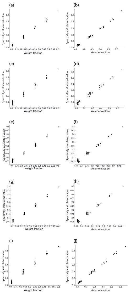
For the plots where the abscissa variable represents the weight fraction, the points corresponding to a given weight fraction of the ingredient lies on a vertical line. The explanation is simple-the samples were made up gravimetrically to prescribed values, thus the actual and the nominal values of weight fraction are all the same (within experimental error) for a given fraction of the specified ingredient. The spectral values plotted on the ordinate direction varied due to the actual changing composition, reflected in the spectral response, hence the data points corresponding to samples of the nominal composition are spread out in only the Y-direction.

For the plots where the abscissa variable represents the volume fraction, the points corresponding to a given volume fraction of the ingredient lie along a line essentially parallel to the direction of the line through all the samples of varying composition. This reflects the improvement of the performance attainable through the use of volume fractions. As we’ve seen previously with the more limited sample set (2), when volume fractions are used as the measure of concentration, the change in value of the constituent concentration is mirrored by an equivalent change in the value of the concentration as determined by the CLS algorithm (2). The calculated values of the concentration measure within each group of data points then follows the trend of the data very nicely, instead of them all lying vertically as in the weight percent values of Figure 3.

The difference between the two cases is that when weight fraction is used for the constituent concentration, the value used to represent concentration of the sample is constant, because the samples were made up that way-to contain a pre-specified amount of the ingredient. In this case, only the spectroscopically calculated value changes (due to the variations in the other components), and therefore the resulting data points fall on a vertical line. When the volume fraction is used as the constituent value, then both the spectroscopically calculated value and known reference value change, and change concurrently, so that the data points for each sample lie on a sloping line that reflects the corresponding changes in the two values.

Another characteristic of the data can also be seen in some (although not all) of the plots in Figure 3. Some of the clusters of data points for the plots of spectral values versus volume fractions show an additional effect. This effect is the spreading of the data points away from the line defining the main direction of the points in each cluster, in this case perpendicular to the line. In some cases (and this is particularly noteworthy for the butanol plots, methanol plots, and to a lesser extent, for dichloropropane plots), the clusters of points are not randomly spaced away from the line defining the direction of the data, but form a pattern. Albeit imperfect, the pattern shows lines of data points within the cluster, each line containing a different number of data points: first one isolated point, then two on a line, then three, then four. The net effect is that for each cluster, the points appear to be contained in a triangular envelope, mimicking, to some extent, the experimental design from which the plots were created.

The cause of this phenomenon is not entirely clear at this time, although suspicion falls on the potential residual interactions between the various chemical components of the samples. The possibility of hydrogen bonding between the two alcohols and the highly polar -C-Cl bonds in the chlorine-containing molecules also seem likely sources of this sort of interaction.

Expanding Beyond CLS: Introducing PCA

CLS is not the only type of data analysis that can be applied to the spectral data without needing constituent values. Principal component analysis (PCA) is a data analysis method that can be applied to the spectra alone, without needing auxiliary constituent information. We have shown in earlier columns (3–8) that a principal component is a least-square estimator of the underlying data, and that, at each stage, it accounts for the maximum amount of variance remaining in the data after all previous components have been used to explain their respective contributions to the measured data values.

This being the case, if the theoretical assumptions underlying the data are valid, it should not be necessary to compute more principal components than there are independent sources of variation affecting the data set being examined. This is effectively the same as saying this reflects the number of degrees of freedom in the data, ignoring the innumerable degrees of freedom that represent the noise content of the spectroscopic data.

In the case of five-component mixtures such as we are dealing with here, you might think that there would be five degrees of freedom in the spectral data. However, since the mixture components must add up to 100% (called closure of the dataset), the concentration of any four components determines the concentration of the fifth; therefore it is not “free” to vary independently. The restriction that the mixture ingredients must add up to 100% removes a degree of freedom from the data. Therefore the spectral data should contain 5 - 1 = 4 degrees of freedom. Ideally, therefore, a five-component mixture should be completely represented by four principal components, ignoring the noise. What we should observe then, upon performing PCA, is that the variance remaining in the spectral data should decrease as each new principal component is computed and the effect of that component is removed from the data set. Furthermore, the early components will account for more variance than later components; the first principal component that is calculated will account for the most variance of the data, while each of the later components will remove less and less. The effect is cumulative, and successive components will remove more and more variance from the data until the first four components are found, at which point the remaining variance should represent the random noise remaining in the data, and that noise should not change by any appreciable amount if more principal components are computed. The remaining variance will then remain almost constant as successive principal components are calculated. Plotting this residual variance as a function of the number of components should therefore approach a very small almost-constant value, once all the non-noise variations of the data are removed by this process. The actual behavior of this data set is shown in Figure 4.

Figure 4: Variance remaining in the set of mixture spectra, as successive principal components are applied to the set of spectral data. Theory tells us that four principal components should be sufficient for all constituents.

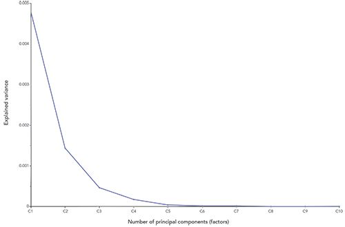
What we actually find in Figure 4, distinct from the theoretical expectation, however, is that there is a continual drop-off of the remaining variance in the data up to at least the sixth principal component. In conformance with theory, the earlier principal components do indeed account for more variance than later ones. Nevertheless, the number of principal components needed to account for or “explain” the spectral data is more than the four degrees of freedom, due to the five individual chemical components that we know are present in the data set (while accounting for the closure of the dataset). The reason for this is also not entirely clear, although it is consistent with the finding, from the examination of the CLS results, of possible interactions between some of the ingredients in the mixtures.

Conclusions (From This and the Previous Column)

CLS analysis of this new data set, which is appreciably larger than the previous data set we were able to use, confirms the results we obtained from the previous data set. The CLS algorithm enabled the reconstruction of the spectra of mixtures from the spectra of the components of each mixture. For several of the constituents (methanol is a good example here), the plot of calculated vs. measured concentration is a straight line when the measured concentration is expressed as volume fraction, but exhibits visible curvature when the concentration is expressed as weight fraction.

Principal component analysis shows that, contrary to theoretical expectation, it requires the calculation and use of more (>6) principal components to account for all the variance in the spectra than theoretical evaluations (four principal components) of the data would suggest (see Figure 4 for the actual amounts of variance explained). Initial explanations for this behavior, based on previous understanding, cast suspicion on more of the “usual suspects”-mainly interactions between ingredients in the mixtures list.

Further, and closer, examination of the results revealed that, while interactions cannot be completely exonerated as a cause of the observed behavior, another unexpected phenomenon showed up, which changes our understanding of how apportionment of variance among several competing effects influences the final results obtained. This phenomenon will be described in a subsequent column.

References

• H. Mark and J. Workman, Spectroscopy 34(6), 16–24 (2019).

• H. Mark, R. Rubinovitz, D. Heaps, P. Gemperline, D. Dahm, and K. Dahm, Appl. Spectrosc. 64(9), 995–1006 (2010).

• H. Mark and J. Workman, Spectroscopy 22(9), 20–29 (2007).

• H. Mark and J. Workman, Spectroscopy 23(2), 30–37 (2008).

• H. Mark and J. Workman, Spectroscopy 23(5), 14–17 (2008).

• H. Mark and J. Workman, Spectroscopy 23(6), 22–24 (2008).

• H. Mark and J. Workman, Spectroscopy 23(10), 24–29 (2008).

• H. Mark and J. Workman, Spectroscopy 24(5), 14–15 (2009).

Jerome Workman Jr. serves on the Editorial Advisory Board of Spectroscopy and is the Senior Technical Editor for LCGC and Spectroscopy. He is also a Certified Core Adjunct Professor at U.S. National University in La Jolla, California. He was formerly the Executive Vice President of Research and Engineering for Unity Scientific and Process Sensors Corporation.

Howard Mark serves on the Editorial Advisory Board of Spectroscopy, and runs a consulting service, Mark Electronics, in Suffern, New York. Direct correspondence to: SpectroscopyEdit@mmhgroup.com