Quantitative Mass Spectrometry: Part II
In this month's installment, columnist Ken Busch continues his discussion of quantitative mass spectrometry with a look at the "cancel out" claim and some of the statistical underpinnings for the proportional comparison of instrument responses for standard knowns and unknowns.

In the first column in this series on quantitative mass spectrometry (MS), we reviewed some of the basic underlying assumptions of the process. We described the various chemical types of standards (Types A, B, and C) after explaining that quantitation will almost always be based upon a proportional instrumental response observed for the known amount of the standard and the response for the unknown. Finally, we briefly described internal and external standards, and stated that internal standards are advantageous because "whatever happens to the unknown target happens to the known standard as well, with the ideal hope that errors will (within the final proportionality comparison) cancel out." I expected emails of disagreement, because the statement is "almost right."

Kenneth L. Busch
In this second column of the five-part series, we now consider the "cancel out" claim and explore some of the statistical underpinnings for the proportional comparison of instrument responses for standard known and unknown, and how those underpinnings should be represented in the classic calibration curve itself. This column is only an overview of a topic that fills thick monographs with the requisite mathematical rigor. However, quantitation is often dealt with only briefly in modern analytical textbooks, and additional review might rekindle appreciation. The actual business of quantitation in MS is the subject of the monographs, many practical handbooks, such as those issued by the Food and Drug Administration (1), or the procedures validated through AOAC, International (2), and ongoing professional certification and education courses. An extensive series in this magazine called "Chemometrics in Spectroscopy" by Workman and Mark describes statistical tools that deal with many aspects of quantitation; a recent book by the same authors has appeared (3). A classic monograph on statistics in analytical chemistry is that of Miller and Miller (4).
There are two fundamental types of error in an analytical measurement: systematic or determinant errors (representing the difference, in either direction, between the measured value and the true value; and random errors (representing the differences in either direction of each individual measurement from the mean of the population of measurements). An erroneous impression is sometimes gained by students that systematic errors are all in the same "direction," but such errors can bias a measurement in either direction from the true value. The magnitude of systematic errors determines the accuracy of a measurement, while the magnitude of random errors determines the precision or reproducibility of a reported value. A reported value can be precise but inaccurate. A reported value can be accurate but imprecise. Finally, it must be made clear that a reported value should represent the end result of a series of measurements recorded under the same conditions. Practical chemists remember that the desiderata of replicate measurements is balanced against the reality of resources such as time, money, and large numbers of samples coming in the laboratory door.
The perceived advantage for an internal standard for quantitative mass spectrometry relates primarily to systematic errors. Using an internal standard does not mean that these systematic errors "cancel out," meaning that any negative error is counterbalanced by some positive effect, and vice versa. Rather, the advantage of an internal standard is that the process is designed such that the sum of all systematic errors is very close to the same magnitude for the standard as for the unknown. When the process is properly validated, the analyst has some assurance that the proportionality factor between response and amount for the standard will be valid for the unknown as well. Remember that the internal standard and the unknown should be present in a well-mixed homogeneous solution (usually liquid). Loss mechanisms are therefore analogous, as are matrix effects (which can be positive or negative). Operator errors (transfer loss, dilution error, and so forth) then affect both the standard and the unknown in parallel. Instability in the solution would affect the standard and the unknown similarly, especially if the standard is of Type A, an isotopically labeled compound. Instrumental drift affects the response for both standard and unknown equally. The systematic errors that affect standard and unknown should be most similar when the amounts of each are very close, because the magnitude of some systematic errors can be a function of the amount of sample present.
In theory, any systematic error could be investigated and attributed to a specific cause. In quantitative MS, sample losses, for example, related to sample preparation (processes including extraction, concentration, homogenization, centrifugation, filtration, derivatization, and dilution) could be traced. Sample loss also occurs in injection of sample onto a gas chromatography (GC) column, and on-column losses have been studied. Transfer lines between chromatograph and mass spectrometer are not 100% efficient. The ionization process in the source of the mass spectrometer is not 100% efficient, and its response also can vary as the nature of the sample bolus changes. Common sense and good laboratory practice describe many of our laboratory procedures designed to minimize losses, but we can never achieve 100% efficiency, even with careful attention to detail (5). Use of the internal standard allows the losses to be compensated for within the proportionality factor.

Table I: Values for expected sample recoveries as a function of analyte fraction
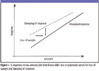
Sample loss is a systematic error that is always in the negative direction. Sample loss is one of many factors convoluted into a metric called sample recovery. If sample loss was the only relevant factor, in theory, sample recoveries should always be 100% (no sample loss) or below. In reality, a calculated recovery of greater than 100% can be valid analytically, representing the universe of systematic errors to include sample preparation and processing. Table I contains values (2) for expected sample recoveries as a function of sample amount. Logically, as the amount of sample decreases and the relative impact of errors increases, the range of expected recoveries widens. Figure 1 illustrates the effect of systematic errors of two types — response dampening and sample loss — in a plot of measured response versus sample amount. The form of the plot is chosen specifically to mirror the classic calibration curve discussed later. Although plot lines such as in Figure 1 might appear roughly parallel over a narrow concentration range, plotting a wider range of sample concentrations might show that the slopes are different, or that the lines are curved at either extreme. The actual measured response-versus-amount curve is shown in bold. Damping of response leads to a lower response than otherwise expected for a known amount of sample (a shift in the negative y direction). Loss of sample generates a systematic error in which more sample is needed to generate a given measured response (a shift in the positive x direction). Use of an internal standard compensates for these shifts due to systematic errors. Note that the shift in the y direction is not a loss of sensitivity; sensitivity is explicitly defined as the slope of the line for the response-versus-amount curve.

Figure 1
The second type of error is a random error. The population of random errors in a replicate determination will trace a normal distribution curve. For a set of n replicate measurements, half will be below the mean value, and half above the mean value, and the distribution of individual measurement values around the mean value will be symmetric. Given this distribution, a standard deviation value (sigma) is derived, providing the means to relate the area under the curve (exactly described mathematically) to the percentage of replicate measurements expected to be within a certain range of the mean value. For example, 95% of measurements, randomly distributed, will lie within one standard deviation on either side of the mean value.
There are different types of random errors (we will see that some might not be random after all) in quantitative MS. The errors can be subdivided under topics of repeatability, intermediate precision, and reproducibility. Each of these terms has an agreed-upon meaning in the community. Repeatability is a short-term function, and the most mathematically compliant. For example, on a single day, on a stable instrument, with a known automated protocol or the same experienced instrument operator, repeatability reflects the truly random variation in sequential measurements of the same sample solution concentration. This delimited situation generates the expected normal distribution curve, with its associated mean and standard deviation metrics. Repeatability also can refer to the result for an unknown obtained after a series of replicate measurements are made (on the same instrument by the same operator) across a range of concentrations, with the result determined by use of a calibration curve. Because random errors occur at each standard point used to determine the calibration curve, the equation of the line calculated from a regression equation can vary slightly, leading to a distribution of values for the same observed response for the unknown. That variation also is codified in the mean and the standard deviation, and often is expressed as a relative standard deviation (RSD). On the quintessential "good day" in an analytical laboratory, RSD for most quantitative experiments can be a few percent. RSD can rise to 10–15% for less well controlled experiments, or using procedures that are not fully validated. As always, should the RSD value rise unexpectedly, the analyst should consider the possibility of new systematic errors.
The RSD for quantitative results from the laboratory on Friday afternoon might not match the RSD of those from Monday (assuming human operators and an attractive weekend on the immediate horizon). The human factor is removed through the use of automation, which can lead to decreased RSD. Still, results from a single laboratory using nominally the same procedure vary over a period of days to weeks, and this variation is the contributor to the intermediate precision. These variations might be due to changes in instrument stability, or to changes in reagents or supplies (even those identical in specifications).
Finally, reproducibility, as a term, is defined as the precision achieved for the same measurement completed by different laboratories. The ideal validated process will lead to the same result from different laboratories, but the reality is that the RSD is expected to grow larger. Remember that an analytical measurement is the end result of an experimental "performance." Just as in the performance of a symphony, even with the same score, and the same notes, different instruments, conductors, different players, and a different "music" hall will invariably lead to a slightly different nuanced performance. With careful cross-validating work, some of those differences can be traced to their sources and could therefore become correctable systematic errors.
External standards in quantitative mass spectrometry are used to construct a calibration curve, which is a response-versus-amount plot similar in appearance to Figure 1. In its simplest sense, a calibration curve is a visual display of the proportionality between measured response and known amounts of external standard. It is constructed based upon the repetitive analysis of each of several standards across a range of concentrations that will span the expected concentration of the unknown sample. Although there are also random errors associated with the "known" amounts of the external standards, we assume for the purposes of this discussion that these values are known exactly, and we will deal with random errors only in the measurement of response. This assumption should reinforce the need for the analyst to exercise great care in the preparation, storage, and use of standard solutions. For example, a standard method for analysis of volatile organic compounds by GC–MS discussed the proper preparation and storage and certification of standards in great detail (6). From a statistics viewpoint, each of the standards themselves should be prepared in an independent fashion (7). Remember that the response measured can be the intensity of an ion of one particular mass-to-charge ratio (m/z), or the summed intensity for a set of ions, or the peak height, or peak area for a data set recorded in a GC–MS run, which is a total ion current trace.
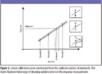
Analysts seem to display a preference for a linear calibration curve such as that shown in Figure 2, which illustrates a direct proportionality between response and sample amount. The phrase "linear calibration curve," although somewhat of a non sequitur, is used widely. How are random errors shown in a response-versus-amount curve? The insets to the right of Figure 2, a simple calibration curve, show three methods. The topmost inset shows that all measured values can be plotted on the graph. The middle inset shows error bars that typically denote the 95% values for that measurement. Specifically, the bars encompass the range of response values that will accommodate 95% of the expected measurements for that standard, according to the statistics of the normal distribution curve. Finally, the bottom inset shows that the random error can be shown by plotting a normal distribution curve itself, distributed along the y axis. Each of the values for each of the standards in Figure 2 is shown with the 95% error bar, which may vary in absolute size depending upon the measurements themselves.

Figure 2
How is the "best" line that links the points for the three standards shown in Figure 2 determined? Note that the point would be moot if there were only responses measured for two standards. A mathematically exact approach is taken, based upon simple statistics. The common regression equations are preprogrammed into calculators and appear in computer spreadsheet programs. Clicking on "Help" in Excel, for example, will link to a tutorial on regression analysis. In the case of Figure 2, for which we assumed that x (the amount of sample) was an independent variable, and y (the observed response) was a dependent variable, a line of equation y = mx + b (m is the slope of the line, and b is the y intercept) can be calculated to represent the ideal "model" behavior that we assume to be true. The regression analysis minimizes the summed offsets of the actual measured points from the ideal line. This "linear least squares" regression analysis is described in more detail (but still without a great deal of math) in the next column, along with concordant regression analyses for idealized behaviors that are not linear.
We use the linear least squares regression to provide the calibration curve, which we can use graphically to provide the answer for the unknown sample. Given a mean response observed for the unknown sample, we draw the horizontal line as shown in Figure 2, and then drop from the intersection of that line with the calibration curve to generate the quantitative result for the unknown. But while the solid line shown in the figure is the "best" line, at a 95% confidence limit, we can draw many lines that intersect all three error bars shown. Assuming an independence of standards, we can draw top and bottom lines that connect the error bars. Then, the horizontal line for the response of the unknown intersects two lines, which, when projected onto the x-axis, provides a graphical estimate of the error in the quantitative determination of the unknown.
For those with interest, the story of who "discovered" linear least squares, complete with issues of priority and/or lack of appropriate citation, has generated some discussion (8–10).
Kenneth L. Busch observes abbreviated reporting of analytical results in the popular media and wonders how the audience assesses the accuracy and precision of the results, and how the audience then uses the information. He explores scientific journals with a critical eye, and gathered examples of "almost right" quantitation until the folder overflowed. This column represents the views of the author and not those of the National Science Foundation. KLB can be reached at wyvernassoc@yahoo.com
References
(1) U.S. Food and Drug Administration, "General Principles of Validation," Center for Drug Evaluation and Research, May 1987.
(2) AOAC Peer Verified methods program, Manual on Policies and Procedures, Arlington, Virginia, November 1993 (see www.aoac.org).
(3) H. Mark and J. Workman, Chemometrics in Spectroscopy (Academic Press, Elsevier, Burlington, Massachusetts, 2007).
(4) J.C. Miller and J.N. Miller, Statistics for Analytical Chemistry, third edition (Prentice Hall, Upper Saddle River, New Jersey, 1993).
(5) S. Jesperson, G. Talbo, and P. Roepstorff, Biological Mass Spectrometry 212(1), 77–81 (1993).
(6) Method 8260C; Volatile Organic Compounds by Gas Chromatography/Mass Spectrometry (GC/MS).
(7) A. Hubaux and G. Vos, Anal. Chem. 42(8), 849 (1970).
(8) J. Dutka, Archive for History of Exact Sciences 41(2), 171–184 (1990).
(9) J. Dutka, Archive for History of Exact Sciences 49(4), 355–370 (1996).
(10) B. Hayes, American Scientist 90(6), 499–502 (2002).
High-Speed Laser MS for Precise, Prep-Free Environmental Particle Tracking
April 21st 2025Scientists at Oak Ridge National Laboratory have demonstrated that a fast, laser-based mass spectrometry method—LA-ICP-TOF-MS—can accurately detect and identify airborne environmental particles, including toxic metal particles like ruthenium, without the need for complex sample preparation. The work offers a breakthrough in rapid, high-resolution analysis of environmental pollutants.
The Fundamental Role of Advanced Hyphenated Techniques in Lithium-Ion Battery Research
December 4th 2024Spectroscopy spoke with Uwe Karst, a full professor at the University of Münster in the Institute of Inorganic and Analytical Chemistry, to discuss his research on hyphenated analytical techniques in battery research.
Mass Spectrometry for Forensic Analysis: An Interview with Glen Jackson
November 27th 2024As part of “The Future of Forensic Analysis” content series, Spectroscopy sat down with Glen P. Jackson of West Virginia University to talk about the historical development of mass spectrometry in forensic analysis.
Detecting Cancer Biomarkers in Canines: An Interview with Landulfo Silveira Jr.
November 5th 2024Spectroscopy sat down with Landulfo Silveira Jr. of Universidade Anhembi Morumbi-UAM and Center for Innovation, Technology and Education-CITÉ (São Paulo, Brazil) to talk about his team’s latest research using Raman spectroscopy to detect biomarkers of cancer in canine sera.
